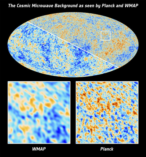
The full sky Cosmic Microwave Background as imaged by the Planck satellite (upper right half) and by its predecessor, NASA’s Wilkinson Microwave Anisotropy Probe (lower left half). Credit: ESA and the Planck Collaboration; NASA / WMAP Science Team
The spring in the Northern Hemisphere brought along the primordial seeds of the Universe. The Planck satellite has completed precise measurements of the fluctuations in the temperature of the Cosmic Microwave Background (CMB), radiation emitted when the Universe was ~380,000 yrs old. How precise? So precise that the error bars on the temperature fluctuations measured are not determined by instrumental noise, but rather by the systematics caused by astrophysical processes. This is to say that the Planck team spent a huge amount of time trying to remove foregrounds from their data: Galactic and extragalactic astrophysical sources that, while interesting by themselves, contaminate CMB measurements by interacting with the CMB photons on their way to us. The angular resolution of the CMB map is roughly 7 arcminutes and the accuracy on the temperature fluctuations measured is of the order of 10-6. The Planck collaboration announced their results on March 21st, presenting their new constraints on cosmological parameters and making data products available to the scientific community. In an upcoming data release in early 2014, the Planck team will provide the full temperature and polarization data. In this post, we summarize two of the papers released by the collaboration on Thursday.
Remarkable agreement with ΛCDM, plus a few puzzles
Title: Planck 2013 results. I. Overview of products and scientific results
Authors: Planck Collaboration
The Planck collaboration’s main goal, first defined in 1995, is to map the temperature fluctuations of the CMB with unprecedented sensitivity, and in turn, determine the cosmological parameters of the Universe with great precision. With roughly 3 times better resolution and 25 times better sensitivity than its predecessor, NASA’s Wilkinson Microwave Anisotropy Probe (WMAP), the Planck collaboration has made substantial progress towards achieving these goals with its first data release. The major cosmological conclusion reached by Planck is that their data agrees remarkably well with the standard, six parameter cosmological model known as ΛCDM (described in terms of the 9-year WMAP results in this astrobite). The Planck team has measured the CMB angular power spectrum, which describes the amplitude of the temperature fluctuations as a function of scale on the sky. Generally, the power spectrum is plotted as a function of multipole number ℓ, where small ℓ corresponds to large scales on the sky. As evidenced by the figure below, the six parameter ΛCDM model not only provides an excellent fit to the Planck spectrum, but also to the 9-year data from WMAP and the smaller scale CMB data from the Atacama Cosmology Telescope and the South Pole Telescope.
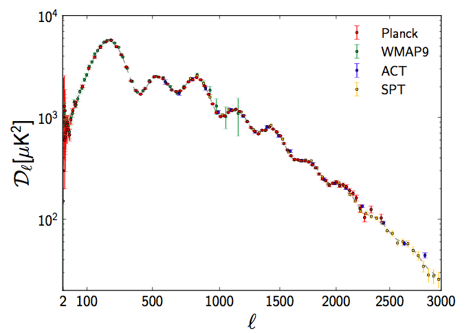
The measured angular power spectrum from Planck, the 9 year WMAP data, the Atacama Cosmology Telescope (ACT), and the South Pole Telescope (SPT). The best fit cosmology found by Planck provides an excellent fit to all four data sets. (Fig. 25 of Planck Paper I)
While the same ΛCDM model describes the Planck data well overall, there are some significant changes in parameters from previous estimates. In particular, the Planck results indicate about 6% less dark energy, 9% more normal matter, and 18% more dark matter in comparison to previous CMB results. The results also indicate that the expansion of the Universe, characterized by the Hubble constant Ho, is proceeding slightly slower than expected from previous measurements. Perhaps most intriguing, the Planck team confirms the presence of some large scale anomalies in their temperature data, which were first detected with WMAP. No current theoretical models can sufficiently describe the origin of these anomalies, and these findings will surely ignite a flurry of theoretical work. Lastly, the Planck data detects the gravitational lensing of the CMB at extremely high significance and finds strong evidence for the occurrence of inflation. Keep reading to discover Planck’s constraints on the type of initial density fluctuations that led to the structure we see in the Universe today.
The Gaussian Universe
Title: Planck 2013 results. XXIV. Constraints on primordial non-Gaussianity
Author: Planck Collaboration
One of the big question marks in cosmology is whether the primordial density fluctuations are Gaussian. Gaussianity in this context means that the values of the temperature fluctuations can be drawn from a Gaussian distribution. Deviations from Gaussian conditions allow us to constrain models of the physics of the early Universe. We do so by going beyond the power spectrum statistics (the topic of the previous section).
Any Gaussian random field can be characterized simply by its two-point correlation (and in Fourier space by its power spectrum). If the primordial perturbations evolve non-linearly or if several inflationary fields interact, the CMB temperature fluctuation field would be non-Gaussian. For a non-Gaussian field, it is insufficient to describe it in terms of its power spectrum. We need to compute, at least, the next order statistics, which in Fourier space is called the bispectrum. The usual approach to parametrizing non-Gaussianity is to do so in terms of a non-linearity parameter, fNL. This parameter captures the amplitude of the bispectrum, which is a function of three wavevectors, k1, k2 and k3. Because the three wavevectors must sum to zero, we can visualize contributions to the bispectrum as triangles of different shapes.
The interest in measuring departures from Gaussianity arises because they allow us to set constraints on the mechanism of inflation. Different inflationary models predict different non-Gaussian effects, described not only by the amplitude of the bispectrum, but also by which triangle shapes most contribute to the bispectrum and on which scales they do so. For example, in the limit where k1 << k2 ~ k3, the “squeezed limit”, if significant non-Gaussianity is detected, it would rule out single-field slow-roll inflationary models in favor of multi-field inflation. “Squeezed” non-gaussianity is also predicted in cyclic and ekpyrotic models. One example of inflationary model that peaks in the “equilateral” shape, for which k1 ~ k2 ~ k3, is DBI inflation. The “orthogonal” shape is a feature of generalized single-field models or Galileon inflation. Planck has set the most stringent constraints in non-Gaussianity thus far, finding that their data is consistent with a Gaussian Universe. For the shapes we described above, they obtain the following constraints,
An impressive amount of work has gone into checking the consistency of these results by resorting to different estimators, validated through numerical simulations, and into removing contaminants. They have furthermore performed a model-independent reconstruction of the bispectrum (instead of looking at particular triangle shapes) and set constrains on higher-order statistics, the trispectrum, which we have not discussed here. In this post, we have only referred to several specific models of inflation; for a more detailed discussion on the impact of the Planck CMB measurements on constraining the parameter space of inflationary models, refer to the Planck collaboration paper.
I would like to mention Liu & Li’s work on
http://arxiv.org/abs/0907.2731
which derived the similar cosmology parameter as Planck’s while using WMAP data (but with different process procedures) several years ago.
I don’t think so. Although the matter and dark energy density parameters Liu&Li derived are similar to the Planck results, the sigma_8 and Hubble parameters are off.
The new cosmological parameters are remarkably similar to those in Ken Croswell’s 2001 book The Universe of Midnight (page 241):
Hubble constant: 65 (Croswell) versus 67 (Planck)
Omega: 0.3 (Croswell) versus 0.315 (Planck)
Lambda: 0.7 (Croswell) versus 0.685 (Planck)
It will be interesting to see how these parameters change after Planck obtains more data.
I am not familiar with the book you are referring to, but the parameters you quote are a typical choice when one is trying to compute order of magnitude estimates of cosmological observables. Does the author quote a source and/or error bars?
Hello scientists,
is anyone of you so kind to define or better to explain to a dummy what are Angular Power Spectra? I read explanations in english and in my native language german with no success.
I cannot imagine, where those angulars are (circle,sphere?). Isn´t there a simple graphical model for example?
Regards from Germany
Klaus Lang
Hi Klaus,
Hopefully this isn’t too technical but since it’s a technical topic it’s sometimes necessary to rely on technical concepts to get the point across.
First, think about some function, plotted as a function of only variable, call it x. This could be any arbitrary curve. It turns out that this curve, no matter what it is, can be written as the sum of an infinite number of sine and cosine functions. This is what’s known as Fourier analysis, Each function will have a different frequency, that is, they will have a different shape. Low frequency sine waves go up and down slowly, while high frequency waves go up and down much more quickly.
A power spectrum is just a way of writing down how much of any particular frequency will contribute to the infinite sum of sines and cosines. More formally, the power spectrum is the Fourier transform of the curve.
Now, what is an angular power spectrum? Well, the sky is two dimensional, so we need to use a different set of functions than just sines and cosines. It turns out that the natural choice are the spherical harmonic functions. The CMB power spectrum tells you how much each spherical harmonic function contributes to the CMB signal we measure on the sky. The power spectrum is in some sense the Fourier transform of the CMB map.
Thank you Nathan,
I will think about your explanation, but it´s hard to understand for me.
I am afraid, I will never understand this stuff. It makes me sad.
For example: why is the sky two dimensional?
And where “my” angels?
I think it is a matter of the spherical harmonic functions.
Regards from Germany
Klaus Lang