- Title: KIC 3858884: a hybrid δ Sct pulsator in a highly eccentric eclipsing binary
- Authors: C. Maceroni, H. Lehmann, R. da Silva, et al.
- First Authors Institution: INAF
- Paper Status: Accepted for publication in Astronomy & Astrophysics
If you read Astrobites regularly, or even semi-regularly, you understand the importance of the Kepler mission to discovering exoplanets. But Kepler, which observed ~100,000 stars continuously for over 3 years, has also uncovered many other interesting stellar systems and properties. Cataclysmic Variables and pulsating stars are just two examples, as well as a new way to measure surface gravity. The paper we will discuss today describes a pulsating Delta Scuti star in an eclipsing binary with another star.
Stellar pulsations are important because they can help shed light on the internal composition and structure of stars through the application of asteroseismology. Delta Scuti stars are one type of pulsating star that lie in the instability strip of the Hertzsprung-Russell Diagram, a nearly vertical region where nearly all pulsating stars are found. Other pulsating stars such as RR Lyrae and Cepheids are also found along the instability strip. Delta Scuti’s have both radial and non-radial pulsations. Radial pulsations occur when the star expands and contracts uniformly, like a beach ball you alternately inflate and deflate. Non-radial pulsations occur when the pulsations travel in other directions, such as around the star or alternating between hemispheres. For most Delta Scuti stars, their pulsations are between 0.03 and 0.3 days. Check out Zach’s post for more details on pulstions in Delta Scuti stars.
The authors studied a Delta Scuti star in an eclipsing binary, meaning one star passes in front of the other from our point of view. The Kepler data yields beautiful, uninterrupted photometry of the system that helps to disentangle the various pulsational modes. The authors also collected spectroscopy of the system to measure radial velocities and abundances of various elements. The photometry and spectroscopy were used to measure the mass, radius, orbital separation, pulsations, effective temperature, and surface gravities of the stars. It turned out that these two stars are very similar, with only small differences in radius and effective temperature.
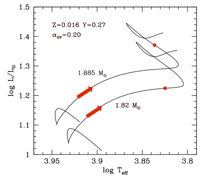
Figure 1: An example of possible evolutionary tracks for the two stars, based on the models. These tracks were selected because the properties of both stars are in agreement with the observations. The arrows shows the direction the stars evolve along the paths. Y is the fraction of helium in the atmosphere of the star. Z is the fraction of heavier elements.
Once the physical parameters of the two stars were determined, the authors tried to understand the evolutionary history of this system. They did this by examining simulations of stellar evolution in which they could vary multiple parameters, including the masses, abundances, temperatures, and radii. The photometry and spectroscopy place constraints on these parameters, which help the authors chose possible evolutionary tracks.
Figure 1 shows one of the possible evolutionary track from the models. The two lines represent the path each star is following. Both stars started in the bottom of the plot, then moved along the path indicated by the arrows to where they are today, represented by the red dots. In the future, they will continue to move along the lines. Despite how close they are in mass, the slightly more massive star is more evolved, as indicated by its more advanced position along the path.
Because of the similar properties, but slightly different evolutionary stages, this system will provide nice information on the evolution of stars in this mass range and around the instability strip. Further analysis of the pulsations of the Delta Scuti will enlighten whether some of the pulsations are caused by tidal forces from the other star.
Very interesting astrobite. But I have difficulty understanding what the axes on the chart refer to. Obviously luminosity and effective temperature, but I (a Bear of Little Brain who is trying to catch up on mathematics whilst teaching her elderly brain astronomy) could really do with it being spelt out…
Especially the x-axis.
If you have time…. I’d be everso grateful!
Margarita
Margarita, thanks for the comment and apologies for not explaining that better up above. You are correct that the axes are luminosity and effective temperature. Luminosity refers to the total energy output from an astronomical source, in this case stars. In this plot, that number is divided by the luminosity of the Sun. The effective temperature of a star can be thought of as the average temperature that we can observe in the atmosphere of a star. We can’t see all the way down to cores of stars, where is it much hotter; we can only see a small way into the atmosphere. The official, more technical, definition is that the effective temperature is the temperature of a blackbody, a perfectly emitting source, that has the same luminosity and radius as the star.
Hope this helps!
Many thanks, Josh, for responding – I really appreciate it!
Do you think that you could explain a bit more about what the figures on the x-axis (3.8 to 3.95) refer to?
I know that that axis is effective (blackbody) temperature and that the usual H-R diagram goes cooler to hotter stars right to left.
This chart says it’s a logarithmic scale, but whereas the y-scale log is a straightforward common log (base 10), the x-axis doesn’t SEEM to be the common logarithm.
I got a bit of background info from the arXiv abstract (http://arxiv.org/abs/1401.3130 KIC 3858884: a hybrid δ Sct pulsator in a highly eccentric eclipsing binary), which gave the temperatures as 6800 and 6600K.
(” The binary components have very similar masses (1.88 and 1.86 Msun) and effective temperatures (6800 and 6600 K), but different radii (3.45 and 3.05 Rsun). “)
If be so grateful if you COULD explain how those x-axis figures are derived and what the log base is. It’s probably obvious, and I’m not “seeing for looking”!
Many thanks again,
Margarita
PS. I would have been back here sooner, but the alert notice didn’t arrive. (Tho the regular astrobites notices have.) Fortunately, I decided to double check the website today and found your comment.
Margarita,
You are actually correct, the x-axis is log base 10 as well. As you said, the current temperatures are ~6800 K and log(6800) = 3.83, which is about where the red points signifying the current state of the stars lie.
You are also correct that the x-axis is backwards from what most people expect, with hotter temperatures on the left and cooler temperatures on the right. For this plot, it ranges from ~8900 K down to ~6300 K.
Cheers
Josh
Again, many thanks, Josh, for your patience and your explanation.
And sorry to have been stupid! If I had just thought to check what log(10) of 6800 was, it would have been obvious. I think that I was fixated on the rather peculiar logarithmic scale that expresses stellar magnitudes and was trying to fit the numbers to that!
Best wishes, and many thanks to you and your colleagues for astrobites – they are so helpful.
Margarita