Title: Spectral analysis of Uranus’ 2014 bright storm with VLT/SINFONI
Authors: P. G. J. Irwin, L.N. Fletcher, P.L. Read, D.Tice
First Author’s Institution: University of Oxford
Paper Status: Submitted to Icarus
After NASA’s Voyager 2 observation in the 1980s, we thought Uranus’ atmosphere was relatively static due to the absence of atmospheric features. When detailed maps of Uranus were finally made possible in the 1990s/2000s with the development of large ground based telescopes and more sophisticated optical techniques, the picture become much more complicated. As one would expect (since nothing in space sciences is ever static), these detailed maps revealed a dynamically active atmosphere with several mid-latitude clouds. This drove several amateur astronomers to point their telescopes at Uranus in order to detect the cloud features themselves. In September 2014, a couple of these amateur astronomers noticed what seemed to be an incredibly bright storm in atmosphere of Uranus. Within months, an international campaign had begun to explain the dynamics of this phenomenon. Today’s astrobites reveals the analysis of these observations. Not only is this a great result scientifically, it is also an exceptional example of how science (space sciences) is capable of uniting people from around the world under a common goal. In this case everyone wants to know: what in the world is going on with Uranus?
Just one month after the storm was spotted, Irwin et al. got observing time on the Southern European Observatory’s (ESO) Very Large Telescope (VLT). In order to fully understand the intricacies of what was going on, they needed not only high spectral resolution but also spatial resolution. Spectral resolution dictates how many data points you get over a certain wavelength range. Spatial resolution is a trickier concept to visualize. If you picture your observation of Uranus as a 2-dimensional image, ideally you would need several pixels to cover the surface area of Uranus. The more pixels you get, the higher spatial resolution you attain and the clearer our image becomes. With VLT’s spectrograph SINFONI, the observers were able to attain 2048 individual spectra, each with 2048 wavelengths, covering the range 1.436-1.863 microns. For those that don’t have the electromagnetic spectrum memorized, this corresponds to infrared light and together allow the observers to make detailed maps of Uranus’ cloud layers.
The product of these intricate observations is shown in the false color images below. Right away you can see the stark bright spot in each of the panels. The upper row are observations taken on the 31st of October at two different time intervals and the bottom row are observations taken two weeks later, also at two different time intervals. In these false color images, the deep clouds appear red, intermediate clouds appear yellow and the high haze clouds appear bluish. The depth of the cloud is determined by looking at the spectroscopy at each pixel, mentioned above. Different wavelengths of light will penetrate different depths of the atmosphere so we can get a pretty good idea of how the clouds are layered.
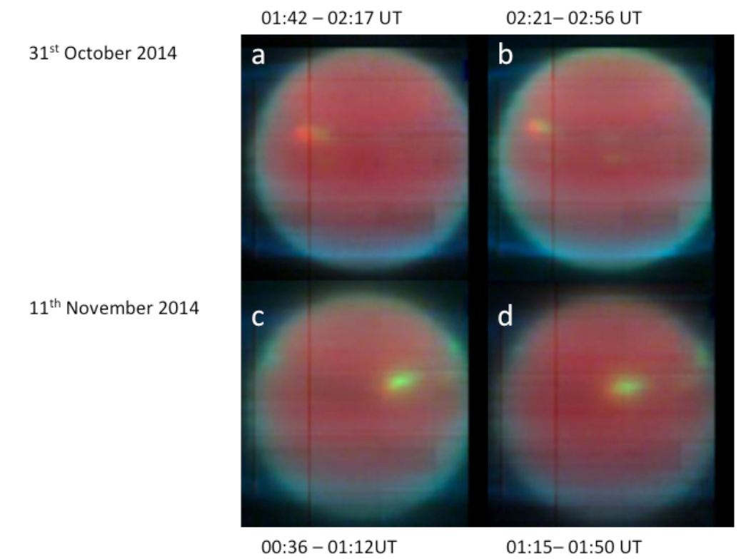
Figure 1. Detailed maps of Uranus’ clouds shown in false color images. The red color corresponds to a deep cloud deck, the yellow color to an intermediate cloud deck and the blue to high hazes in the atmosphere. The cloud is clearly changing as a function of time. From October to November, the cloud becomes more extended and loses it’s faint red center. This means that over time, the cloud became more vertically extended.
From a complex retrieval analysis (which we have previously described here), the authors determined the clouds are most likely made of methane ice particles with the center of the clouds roaring with 100 m/s winds. These observations also give us an idea of the morphology of Uranus’ cloud structure. In the upper panels of Figure 1, there is a small red tint in the middle of the cloud which indicates the center of the storm consists of deeper clouds. Comparing the October observations to the November observations, you can see that the red tint in the middle of the storm goes away and the yellow features thicken. Meaning, those deep clouds we saw in the center of the bright spot originally, turned into more spatially distributed intermediate clouds.
This leads the authors to conclude that the clouds form from deep in the atmosphere where the winds are highest. Very much like a pot of boiling water, the clouds then bubble up to a higher region in the atmosphere where the winds are less severe. So what can we learn from this?
For the most part, we don’t have a fantastic understanding of atmospheric dynamics for the outer Solar System planets. Storm features have been observed on Saturn and Jupiter but never before on Uranus. Furthermore, we still don’t know how exactly these storms come about. Each time we observe another storm, we gain a deeper understanding of general atmospheric dynamics. This will help us tremendously when we attempt to characterize exoplanets. And as it turns out, the history of Uranus observations turns out to be pretty similar to that of exoplanets. GJ 1214b, which was been observationally beaten to death by exoplanet astronomers, has revealed a completely featureless spectrum (exactly like the 1986 observations of Uranus). It’s entirely possible, that as we continue to improve our observations, we will encounter cloud structures similar to those in these observations.