Title: A Posteriori Transit Probabilities
Authors: Daniel J. Stevens and B. Scott Gaudi
Institution: Department of Astronomy, The Ohio State University

Bonus Video: OSU Astronomy Coffee Brief

Transiting exoplanets are the best! Well, I think so, anyways. A transit is the dip in light we see when a planet passes between us and its host star. Transits turn exoplanets into real worlds—we can characterize their atmospheres, bulk compositions, and much else. That’s why little dips in light curves set my heart aflutter. But discovering a transiting exoplanet requires a bit of luck. After all, we can’t observe exoplanetary systems from every direction; we’re stuck on Earth or close to it, so an exoplanet’s orbit needs to be aligned just so for us to view a transit.

How do we find transiting exoplanets? There are two general methods. First, we can look at a plethora of stars at once. The Kepler mission (RIP) observed >150,000 stars continuously for four years. Because Kepler looked at so many stars, it found thousands of transiting planetary candidates. Follow-up observations are difficult, however, because the Kepler stars are relatively faint. Second, we can target planets discovered using radial velocity (RV), hoping to see a transit. These RV planets are scattered all around the sky, so we can’t observe all target stars simultaneously using a single telescope like Kepler—although a future mission (TESS) should change this! Most RV planets won’t transit, but we can extract a huge amount of information from those that do.

What’s the probability that an RV planet will transit? As they (should) teach in kindergarden, a simple estimate is that the probability of a transit is equal to the radius of the host star divided by the semi-major axis of the companion’s orbit. More compactly, P = R/a. This is because the inclination of planetary orbits should be randomly distributed from our point of view. We fit the RV data to find the semi-major axis, a. We can estimate the stellar radius, R, from the stellar spectra we used to measure the RV. Ergo, we know precisely the probability of a transit and thus how many stars we need to target to find a transiting exoplanets… right? Actually, no. As Stevens and Gaudi discuss in this paper, it’s more complicated than that.

The orientation of planetary orbits, in general, should be random. But not all orientations for planets that we detect are equally likely. RV data can’t constrain the mass of an exoplanet independently from its orbital inclination. We only measure a combination of the two, called the “minimum mass.” In reality, planetary masses aren’t distributed evenly; the abundances of super-Earths, Neptunes, and Jupiters are different. So, certain planetary masses are more likely than others and thus our RV planets are more likely to be in some orientations than others. The authors use Bayesian statistics to examine the effects of possible mass distributions on the probabilities that known RV planets will transit. They conclude that exoplanets less massive than Jupiter have up to a ~20% better chance of transiting than previously assumed. This isn’t a huge effect, but it should buoy our optimism for finding transiting exoplanets among RV targets.

The Problem

Our problem with the simple formula (P = R/a) is that it ignores an additional piece of information. Specifically, we’ve also measured the “minimum mass” of the planet with RV. This minimum mass is equal to the actual mass of the companion times the sine of its orbital inclination. Think of it this way: RV measures the back-and-forth motion of the star that we see (in the radial direction). A bigger companion will exert a bigger pull on the star, but the component of motion in the radial direction depends on the orientation of the object. For example, a companion that orbits exactly in the plane of the sky won’t cause any movement in the radial direction no matter how massive it is. At the other extreme, an orbital inclination of 90° corresponds to a system in which the orbit is precisely aligned with our line of sight—a transiting system! The mass of a transiting exoplanet is approximately equal to the measured minimum mass. For misaligned orbits, the actual mass is larger than the minimum mass.

Let’s consider a simple example. Imagine that one Earth-mass was the strict lower limit to the mass distribution; no less-massive exoplanets exist. Now, say that you discovered a RV planet with a minimum mass of 0.1 Earth-masses. You’d know the real mass must be larger than this minimum mass, so the planetary orbit must be misaligned. The probability that this exoplanet will transit is identically zero, regardless of the R and a of the system. Our a priori knowledge of the mass distribution directly affects our knowledge of the orbital alignment.

Unfortunately, we don’t know the real distribution of exoplanetary masses. In fact, that’s currently one of the major goals of exoplanet science! But that won’t stop us from speculating. Theorists run simulations of planet formation that predict different mass distributions. These distributions disagree in many respects and won’t be observationally verified for a while. However, most people believe that small planets are intrinsically more abundant than large ones, which is consistent with the Kepler results.

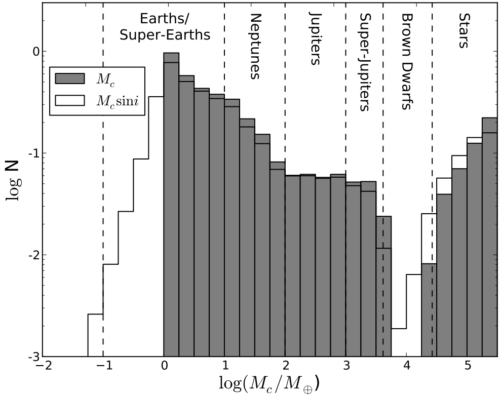
Figure 1: Comparison of the actual mass distribution (filled histogram) to the distribution of minimum masses that we’d observe with a RV survey (empty histogram). If we took the minimum mass distribution as the actual mass distribution, we’d be very wrong. Vertical axis is the number of objects; horizontal axis is companion mass in units of Earth’s mass. (Stevens and Gaudi 2013)

The Solution

At this point, you might be confused. How do we deal with all these nested probabilities? How do we really know what’s really real, in reality? Stevens and Gaudi appeal to Bayesian statistics, a theoretical framework that’s becoming increasingly popular in astrophysics. Bayes’ theorem, simply, states that the probability that a model is true given the data (the posterior) is proportional to the probability that the model would produce the data (the likelihood) times the prior probability that the model is true (the prior). If you understand the Bayesian lingo of posteriors and priors, you’ll get the gist of their paper, even if the algebra remains opaque.

Let’s translate our problem into Bayesian-speak. We care about the actual mass of the planet—that’s the posterior. We know the likelihood that a companion of a given mass will be aligned in such a way to produce the measured minimum mass (P = R/a). We need to think carefully about the prior probability that a given mass distribution exists in reality.

Figure 1 shows a sample mass distribution, assembled from simulations of the formation of planet-sized companions and from studies of the occurrence rate of stellar companions around nearby stars. Again, this is probably wrong in detail; the important point is that it’s not flat. Fig. 1 also shows the resulting distribution of minimum masses as measured with an RV survey on Earth. As you can see, the correspondence between the two distributions depends on the slope of the mass distribution. Where the abundance is relatively insensitive to mass (in the Jupiter zone), the observations basically match reality. But many minimum masses will be measured in a range where no real objects exist (brown dwarfs). Where the mass distribution is sloped, the distributions of the real masses and minimum masses are different—not dramatically so, but enough to make a difference when planning follow-up campaigns to target RV candidates.

The authors then searched the Exoplanets Orbit Database for planets discovered using RV. They computed the posterior probability that each planet would transit, given an underlying mass distribution. They compared these probabilities to those predicted from the simple R/a scaling. They tried two different distributions from the literature, both of which yielded similar results. In particular, planets are more likely to transit than the simple scaling suggests. As seen in Figure 2, a number of planets with relatively large orbital periods have probabilities of transits >10%, even though the simple scaling predicts <1% chances. In other words, a small minimum mass is more likely to be a small planet near-transit than a massive super-Jupiter on a very inclined orbit, since small planets are intrinsically more numerous than large ones. This result should make us more optimistic about conducting surveys of RV targets. Perhaps most importantly, however, this paper highlights the importance of using all your available information to plan observations!

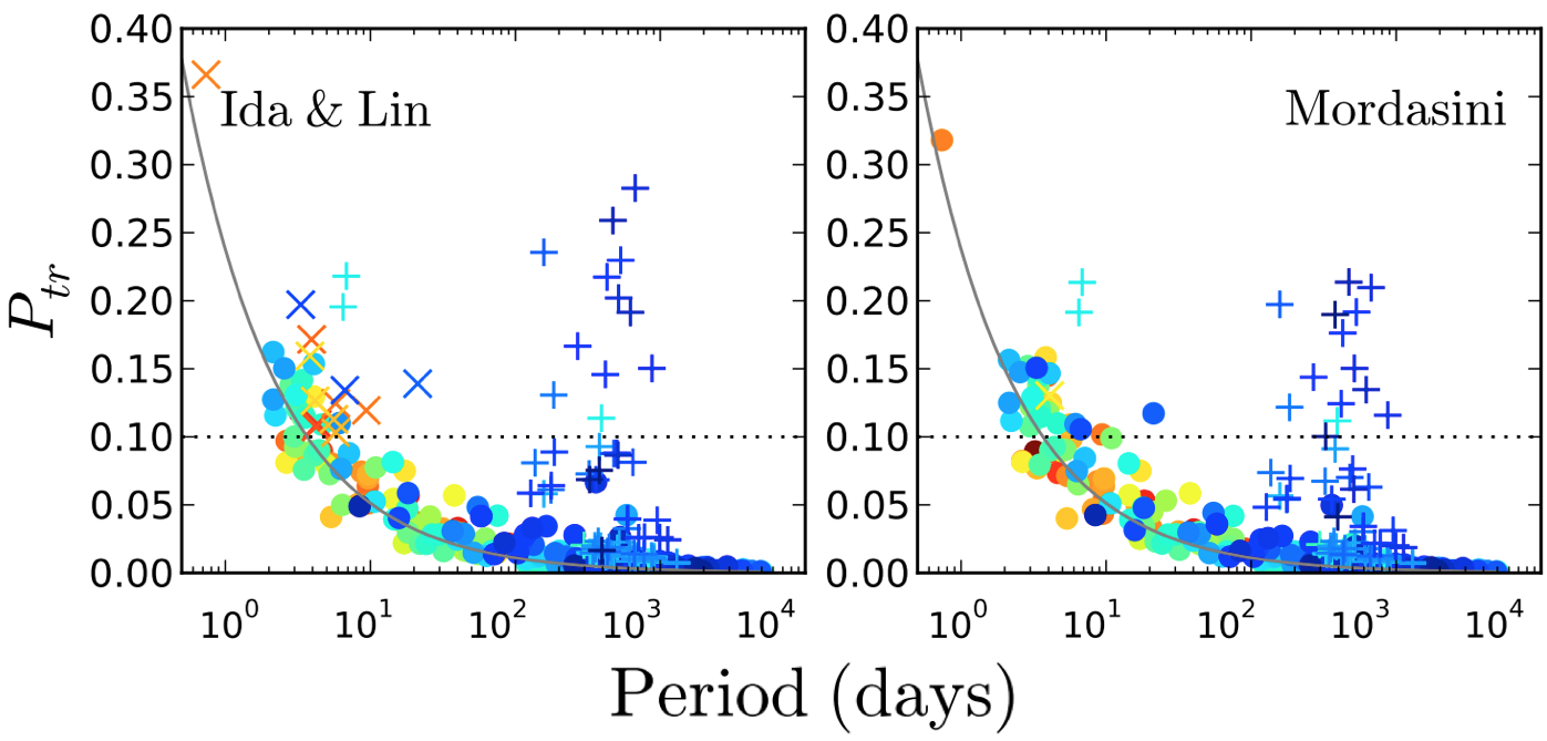
Figure 2: Transit probabilities for RV planets in the exoplanets.org database. Bluer colors indicate more massive planets. Plus signs represent planets orbiting stars with very large radii. The solid grey line is the simple P = R/a scaling and the horizontal dotted line represents planets with a >10% chance of transiting. The simple scaling isn’t horrible, in general, but actual transit probabilities are probably a higher than predicted. (Stevens and Gaudi 2013)

• About the Author

About Joseph O'Rourke

I am a first-year graduate student in planetary science at the California Institute of Technology, where I work with Heather Knutson and David Stevenson. My research interests include the formation of gas giant planets, the internal structures of icy satellites, and the thermo-chemical evolution of terrestrial planets. My favorite planet is Venus and my favorite ice cream flavor is mint chocolate chip. I received my bachelor's degree in Astronomy & Physics and Geology & Geophysics from Yale University in May 2012.

Related posts:

Super-Earths or Mini-Neptunes? Super-Earths or Mini-Neptunes: Part Two Dip-Detection in the Kepler Data MINERVA: MINiature Exoplanet Radial Velocity Array