Title: Evaporation of Planetary Atmospheres due to XUV Illumination by Quasars

Authors: John C. Forbes, Abraham Loeb

First Author’s Institution: Institute for Theory and Computation, Harvard University, Cambridge, MA 02138, USA

Status: Submitted to MNRAS [open access]

Earth-like life is pickier than Goldilocks

Life on Earth: beautiful, wondrous, and utterly at the mercy of the environment.  There are a number of crucial qualities – liquid water, breathable air, temperate sunlight – that we Earth-born life forms need to survive.  Without them, we’d have a truly frightening apocalypse on our hands (worse than any other apocalypse you might have come across).

In light of that, astronomers searching for life (as we know it) beyond Earth look for exoplanets that have these same crucial qualities.  But for an exoplanet to house Earth-like life, there’s quite a lot that needs to be “just right”.  The exoplanet must be in some sort of habitable zone, for example, where liquid water can exist, and the exoplanet must also have some form of hospitable atmosphere.  And just as things can go “just right” to cultivate these qualities, other things can go very wrong.

The authors of today’s astrobite look into one of these characteristics that could go very wrong: the loss of a planet’s atmosphere.  They explore how quasars can rather literally blow these atmospheres away.

From accretion to atmosphere

First question: what’s a quasar?

In a couple of sentences, a quasar is made up of an actively accreting supermassive black hole at the center of a galaxy.  (Believe it or not, there’s a supermassive black hole at the center of our own galaxy, the Milky Way!  It’s called Sagittarius A*, or Sgr A* for short.)  A quasar produces radiation: as material from the surrounding galaxy accretes onto, or falls into, the black hole, the black hole releases energy as intense radiation.

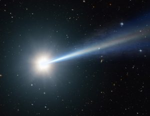
Figure 1: An artist’s gorgeous impression of a quasar. Image credit to NASA/ESA/G. Bacon, STScl.

Second question: what in the universe do quasars have to do with planetary atmospheres?

The answer’s all in the radiation!  Let’s imagine a quasar, like the one depicted in Figure 1.  Intense radiation is flowing outward from this quasar, out into the surrounding galaxy.  Now let’s imagine an exoplanet.  This exoplanet has a lush, tasty atmosphere, and it’s sitting innocently somewhere in this galaxy.  When the radiation from the quasar hits this exoplanet, it warms the exoplanet’s atmosphere, and the atmosphere expands outward.  If the atmosphere gets hot enough, its outer layers can expand so far that they escape the exoplanet’s gravitational field!  And so the poor exoplanet is left with a thinner atmosphere than before.

Today’s authors figured that quasars are the second most important source of radiation for planets (the first most important naturally being the planet’s host star), and thus the second most important objects for this effect.  So they set out to map the connection between the quasar radiation felt by a planet and the planet’s atmospheric loss.  To do so, they fully embraced both theory and statistics.

A collage of calculations

They started with theory.  If we define the following variables:

• M_lost = the total atmospheric mass lost by the planet
• M_p = mass of the planet
• R_p = radius of the planet
• = quasar fluence, which relates to the quasar radiation felt over some span of time

Then, handwaving all of the constants, we can write this nifty approximate proportion:

M_lost  (R_p³ / M_p)

Where we’re making a few simplifying assumptions, such as assuming that a planet hosting life wouldn’t change its bulk density ( M/R) too much over time.

Wrapped up into the fluence are important quasar properties, such as its luminosity and lifetime, as well as the distance of the planet’s system to the quasar.  So based on this proportion, we can pick out some cool relations already: a more luminous quasar, for example, would lead to more atmospheric mass loss, while a more massive planet would lose less of its atmospheric mass.

The authors then turned to the power of statistics.  Basically, they asked the following question: if we point to a random planet in the universe, how much atmospheric mass (based on statistics) do we expect that planet to lose to quasar fluence?

To help answer this question, they mapped out the universe’s fluence distribution – as in, how fluence is distributed across star systems, and thus their planets, in the universe.  This overall distribution involved individual distributions across the universe of a number of both star and galaxy parameters – such as the masses of the host stars, redshifts of the galaxies, and how black hole masses and the bulge masses of galaxies are correlated, just to name a few.

They pieced together each of these individual distributions as a brilliant collage.  One really neat trait about the authors’ work is that they built upon their own theory and calculations and the theory and calculations of other scientists.  It just goes to show the importance of collaboration across different groups, to really make super-cool science come together!

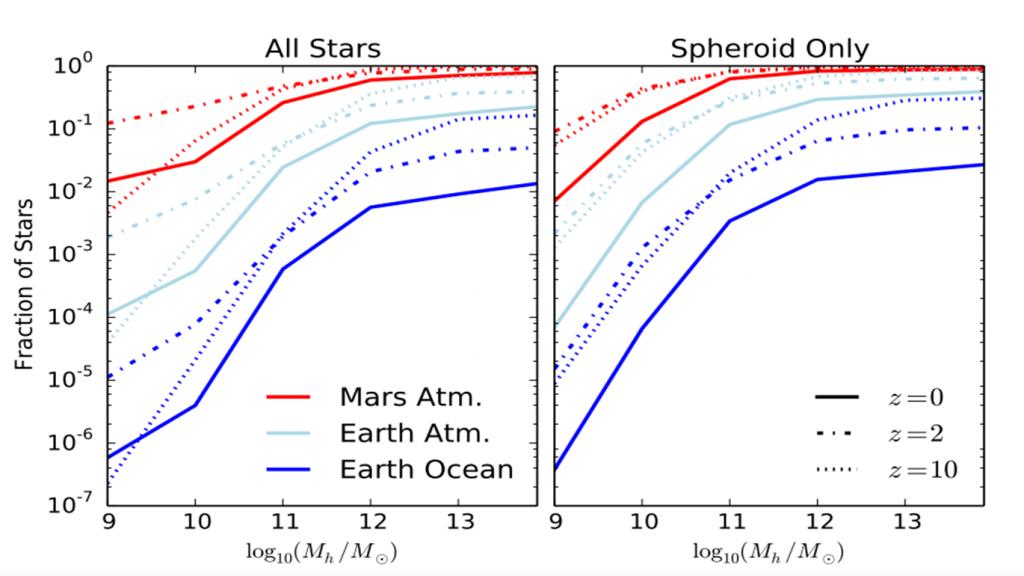
Figure 2: This figure shows the effect of galactic halo mass on planetary atmospheric mass loss. The x-axis gives the logarithm (base 10) of the halo mass, in units of solar masses. The y-axis gives the fraction of stars that have received enough fluence for their planets to lose a given amount of mass, indicated by the colors. (Red is for losing the mass of Mars’s atmosphere, light blue is for losing the mass of Earth’s atmosphere, and dark blue is for losing the mass of Earth’s oceans.) The line style indicates the redshift (z) for that calculation.  (Solid is for z=0, dotted-dashed is for z=2, and dotted is for z=10.) The left plot is for all stars in the galaxies, while the right plot is for just the stars in the galaxies’ spheroidal components. From Figure 4 in the paper.

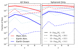
Figure 3: This figure shows the effect of redshift on planetary atmospheric mass loss. The x-axis gives the redshift (z). The y-axis gives the fraction of stars that have received enough fluence for their planets to lose a given amount of mass, indicated by the colors. (Red is for losing the mass of Mars’s atmosphere, light blue is for losing the mass of Earth’s atmosphere, and dark blue is for losing the mass of Earth’s oceans.) The line style indicates the range of logarithmic (base 10) halo masses for that calculation, in units of solar masses.  (Solid is for the range of [10⁸-10¹⁵] solar masses, dashed is for [10¹⁰-10^10.1] solar masses, dotted-dashed is for [10¹²-10^12.1] solar masses, and dotted is for [10¹⁴-10^14.1] solar masses.) The left plot is for all stars in the galaxies, while the right plot is for just the stars in the galaxies’ spheroidal components. From Figure 5 in the paper.

Figures 2 and 3 give examples of their results.  In both figures, the authors use the masses of Mars’s atmosphere, Earth’s atmosphere, and Earth’s oceans as convenient references when considering atmospheric mass loss.  Figure 2 shows that, at any given redshift, as halo mass increases, the fraction of stars that feel enough fluence to drain away any of those convenient reference masses increases.  From this result, the authors point out that planets in more massive galaxies are more likely to feel high quasar fluences.  And from Figure 3, when we look at galaxies with halo masses in the broad range of 10⁸ to 10¹⁵ solar masses, we can see how the fraction of stars exposed to enough fluence to lose the reference masses decreases at higher redshifts.  Over narrower ranges of halo mass, however, we see an opposite, upward trend.

Looking at today’s redshift of zero (see Figure 3!), the authors noted how, based on these statistics, a whopping 50% of the planets in today’s universe may lose enough atmosphere to equal that of Mars.  That’s about kilograms of material, or the weight of about Asian elephants!  About 10% may lose enough atmosphere to equal Earth’s atmosphere (about kilograms, or the weight of around Asian elephants), and about 0.2% may lose enough atmospheric mass to equal that of Earth’s oceans (about kilograms, or the weight of about Asian elephants).

So what do these bleak numbers mean for habitability across the universe?  It’s hard to say!  These statistics may seem grim in the search for Earth-like life, but there could be all sorts of other forms of life out there – forms that maybe don’t need temperate sunlight, for example, or that thrive beneath an ultra-thin atmosphere.  So while possible atmospheric loss is something to keep in mind when we look at snazzy exoplanet systems like TRAPPIST1, we have to remember to stay much more open-minded than Goldilocks to all the wonders the universe has in store.

• About the Author

About Jamila Pegues

Hi there! I'm a 3rd-year grad student at Harvard. I focus on the evolution of protoplanetary disks and extra-solar systems. I like using chemical/structural modeling and theory to explain what we see in observations. I'm also interested in artificial intelligence; I like trying to model processes of decision-making and utility with equations and algorithms. Outside of research, I enjoy running, cooking, reading stuff, and playing board/video games with friends. Fun Fact: I write trashy sci-fi novels! Stay tuned - maybe I'll actually publish one someday!

Related posts:

An Overview of the Extreme Solar Systems III Conference Detecting Transiting Planets Around White Dwarfs The Kepler Exoplanet Census The Radio Activity-Rotation Relation of Ultracool Dwarfs