Title: Asymptotic Properties of Fields and Space-Times

Authors: Roger Penrose

First Author’s Institution: Department of Mathematics, King’s College, London, England [at time of publication – 1963]

Status:  Physical Review Letters (open access)

Nobel prize in physics? More like Nobel prize in astrophysics! Three of the last four Nobel prizes have been for astrophysical work, and each of these prizes has been dedicated to work rooted in the study of spacetime. There are already great astrobites about these (here, here, here, and here), but today we’ll focus not on any particular discovery, but on a related tool for studying spacetime developed in 1963 by one of this year’s Nobel laureates – Roger Penrose (for more on Penrose and the prize, see this bite!). This tool is called the conformal diagram, or the Penrose diagram. The conformal diagram squeezes an infinite spacetime into causally-meaningful finite coordinates – we’ll unpack all these words in today’s bite!

Our place in space(time)

Spacetime is – at its most basic – the set of all 4-dimensional points we can label with coordinates – i.e. names like (t,x,y,z), or (t,r,θ,φ), which are called events. Here we have our familiar spatial coordinates – either cartesian as in the first set of labels or (spherical) polar as in the second – along with a (positive) coordinate t, which gets special treatment as the time coordinate. Spacetime can be flat (as in special relativity) or curved (as in general relativity – and the universe!) and is described in relation to matter inhabiting it by the Einstein equations. We won’t get into all the details of general relativity, but see here for an astrobite-approved introduction!

No matter what country you live in or how lenient your traffic laws, we all have to obey one speed limit – the speed of light. Nothing can move faster than the speed of light, and this introduces a notion of causality – every event is associated with its own notions of past and future. To put this more intuitively (or at least, graphically), physicists employ the concept of a light cone (Fig. 1). A light cone is drawn with the time coordinate t on the vertical axis and spatial coordinates (e.g. x, and y or r and φ) on the other axes. The edge of the cone is the line with a slope given by the speed of light rotated around the origin (the speed of light is often set to c=1 since it is easier to draw lines with slope 1 than with slope 2.998 x 105 km/s). Events are considered to be in the past of an event if they are in the bottom half of the light cone and in the future if they are in the top half of the light cone. This means that events outside the light cone (which are called “spacelike related” – see Fig. 1) can NEVER interact with the event in question! 

This might seem a little weird, but it is just a re-phrasing of our universal speed limit, which can be seen through a quick example. Let’s say your alien friend texts you from Alpha Centauri (which is over 4 light-years away), and let’s call that event e_send = (t_send, r_alien, θ_alien, φ_alien). We can then draw the light cone for that event. Let’s call the event of you getting that message on your interstellar phone e_get =  (t_get, r_you, θ_you, φ_you). If you received that message in less than 4 years, the sending event  (red point) would fall outside of the light cone of the receiving event e_get (such an event is called spacelike related), which is the same as saying the text (red dashed arrow) traveled faster than light! Since this is impossible, e_get has to be in the future light cone of e_send, and e_send has to be in the past light cone of e_get.

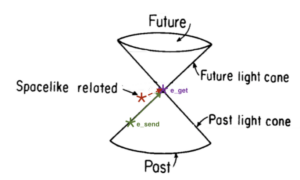
Figure 1: Light cone for an event e_get in spacetime, with key properties labelled. The time direction points upward, while the spatial directions are perpendicular to it. The top half of the lightcone is the future of the event and the bottom half is the past of the event. Points that fall outside the lightcone can never affect or be affected by e_get. The red point corresponds to an impossible event (Adapted from Wald 1984)

Crunch time!

Lightcones are great for thinking about causality for individual events but for interesting spacetimes (like those considered for black holes or cosmology), we want to think about causal relationships for the entire spacetime (which may be curved). This is a problem graphically because, even without all three space dimensions, in our simple lightcone picture we can’t put an infinite amount of spacetime on a finite piece of paper! So, can we represent the infinite nature of spacetime in a finite way that is easier to see and think about? More importantly, can we do this in a way that does not ruin the causal relationship between events? Penrose provides the answer, which, at least sometimes, is yes!

Ignoring causality, how do we “crunch” infinity into a finite diagram? Do we need some dozen-page derivation to tame the unquantifiable infinity? No! All we need is a humble change of coordinates (or relabeling each event) using our old friend the tangent function. The inverse of the tangent function (tan^-1(x)) takes as inputs any real number, but it only outputs values between -π/2 and π/2 (Fig. 2), so in this sense, the inverse tangent function crunches all real numbers into a finite range. This is one of the two key coordinate changes used to draw the conformal diagram.

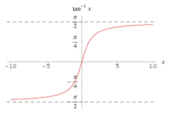
Figure 2: The inverse tangent function (Wolfram Mathworld) – the domain of the function is the whole real line, while the range is restricted to be finite, as indicated by the dashed lines.

Coming back to causality, by a careful choice of labels for our events in spacetime (what are called “null coordinates”) we can enforce that in our final coordinates – the ones used for the diagram – light rays travel at 45-degree angles only. This is the other key coordinate transformation used to build the conformal diagram. By this 45-degree rule, for any point in spacetime we can then confidently draw past and future lightcones that extend to infinity(!) – geometrically demonstrating which other points in the whole spacetime could have affected our point in the past, and which it can affect in the future.

Putting Pen(rose) to paper

Now with the keys of 1. 45-degree light cones, and 2. the crunching function in hand, we can unlock Penrose’s conformal diagram. The left panel of Fig. 3 shows a conformal diagram for flat space (called Minkowski space). Let’s slowly unpack the labels. We begin with polar coordinates for the spacetime (t,r,θ,φ), and perform a set of coordinate changes (including our key 45-degree and crunching changes) on the t, and r coordinates to produce η, and χ, respectively. We have the vertical axis as the coordinate η corresponding to time, and similarly, the coordinate χ corresponding to space on the horizontal axis. Here the angular directions are not shown (but they are still a part of the spacetime). 

Before discussing causality, let’s first discuss the boundaries. By “crunching” we have forced the infinite range of t and r into the boundaries of the diagram. These boundaries are given by a bunch of i’s – at the very bottom of the diagram, i^– is called “past timelike infinity” and, correspondingly i⁺ is “future timelike infinity”.  These are fancy names we won’t precisely define, but they correspond to the minimum and maximum allowed values of our “crunched” coordinates (η,χ)=(-π,0) for i^– and (η,χ)=(π,0) for i⁺.  Similarly, we have “spacelike infinity” i⁰, which corresponds to the point (η,χ)=(0,π). Finally, we have I^– and I⁺, which connect these points, and to which we will briefly return. These new coordinates account for events across the entire spacetime!

Helpfully, there is also a lightcone drawn (with 45-degree angles!) for one of the events in the spacetime. If we were to extend the cone to the boundaries of the diagram, we would then cover ALL possible events that could ever “talk to” the event with the lightcone. This means we have a characterization not just of the entire spacetime, but of causality over the entire spacetime. The boundaries I^– and I⁺ are reflections of the 45-degree rule in the diagram for light cones that begin at i^– and i⁺.

The left panel also shows how our original coordinates t, and r, are deformed by the coordinate changes used to build the conformal diagram. In the original light cone picture, lines of constant t and r would have simply formed a bunch of squares, like regular graph paper. However, the effect of making the coordinate changes, including the crunching and 45-degree-enforcing coordinate changes, have distorted the original coordinates. You might object that the diagram has ruined our original sense of distance – and you’d be right, the conformal diagram does not accurately represent distances in the original coordinates. But the diagram is already representing the causal structure of (infinite) 4-dimensional spacetime in (finite) 2-dimensions – you might consider cutting it some slack! 

Finally, we can appreciate the right portion of the right panel of Fig. 3, which shows Penrose’s original 1963 conformal diagram. All the features we’ve looked at so far are in there: his I points are the left panel’s i points, and his squiggly boundary ℑ’s are the left panel’s boundary I’s. The reason for the visual difference between the left panel and the spinning top-like diagram on the right is that Penrose has additionally rotated the diagram about the χ = 0 axis to produce this top-like structure – the point i⁰ in the left panel traces out the central circle in the right panel. In this way, he has put the φ dimension into the diagram (which is hidden in the left panel) – but the structure of the spacetime is the same as it is in the left panel. The left part of the right panel with the cylinders is related to more technical aspects of the boundary ℑ’s.

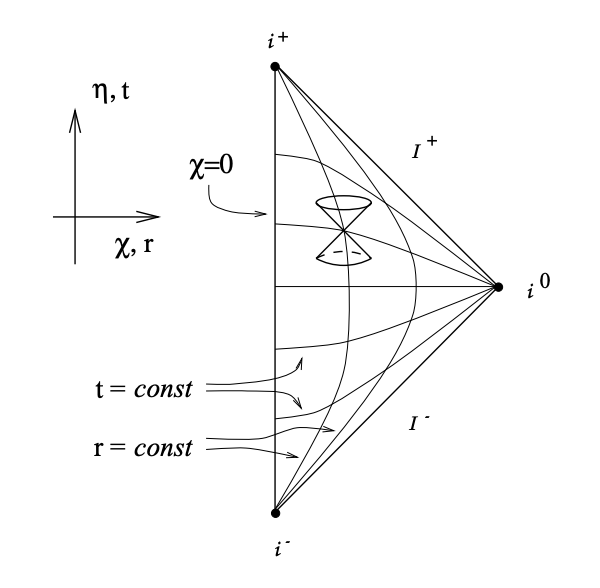
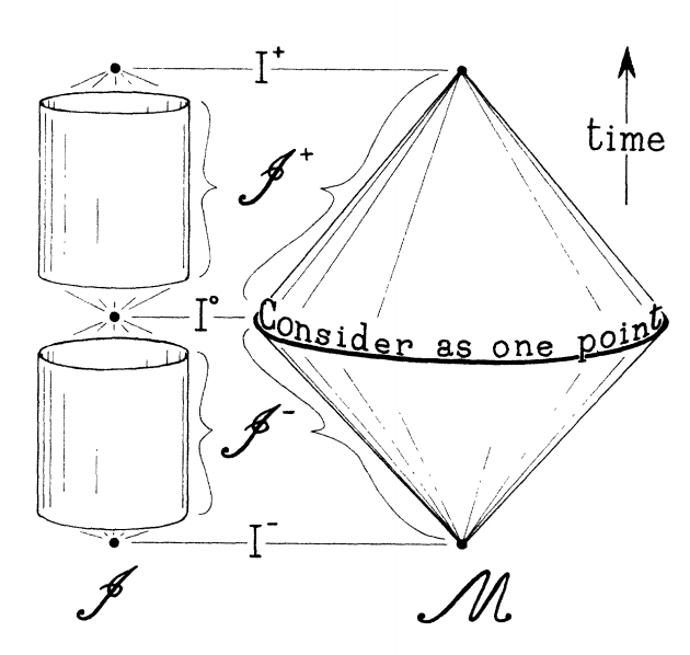
Figure 3: Left: The conformal diagram for flat (Minkowski) spacetime (Carroll 1997). Right: Penrose’s original conformal diagram from 1963 – Fig. 1 of today’s paper.

Diagram schmiagram, what about physics?

So why go to all the trouble of drawing a conformal diagram? Well, the key improvement of Penrose’s diagram over previous versions of spacetime diagrams was the clearer treatment of the causality and points at infinity. Penrose and others used the simplification provided by the diagram to describe what happens to particles crossing the horizon of black holes. The conformal diagram is now widely used in discussing the causal structure of different types of black holes. The diagram can also be used to describe the causal structure of a star as it collapses to form a black hole in the first place. The conformal diagram is also useful for discussing cosmological inflation (see this interactive(!) bite) – in particular, it clearly illustrates the horizon problem posed by observations of the Cosmic Microwave Background. In this case, the conformal diagram shows the entire observable universe up to today. It’s often said that a picture is worth a thousand words – sometimes a diagram is worth infinity!

Astrobite edited by: John Weaver
Featured image credit: Today’s paper

• About the Author

About Jamie Sullivan

I am a third-year astrophysics Ph.D. student at UC Berkeley and part of the Berkeley Center for Cosmological Physics. My current research focuses on measuring and modeling large-scale structure to constrain cosmological parameters. I completed my undergraduate at UT Austin, and am originally from the Washington D.C. area.

Related posts:

The Nobel Prize in Physics 2020: Reinhard Genzel How Plural are Singularities? The First Image of a Black Hole The Nobel Prize in Physics 2020: Roger Penrose