Title: Deconvolution of JWST/MIRI Images: Applications to an AGN Model and GATOS Observations of NGC 5728
Authors: M. T. Leist, C. Packham, D. J. V. Rosario, D. A. Hope, A. Alonso-Herrero, E. K. S. Hicks, S. Hönig, L. Zhang, R. Davies, T. Díaz-Santos, O. Ganzález-Martín, E. Bellocchi, P. G. Boorman, F. Combes, I. García-Bernete, S. García-Burillo, B. García-Lorenzo, H. Haidar, K. Ichikawa, M. Imanishi, S. M. Jefferies, Á. Labiano, N. A. Levenson, R. Nikutta, M. Pereira-Santaella, C. Ramos Almedia, C. Ricci, D. Rigopoulou, W. Schaefer, M. Stalevski, M. J. Ward, L. Fuller, T. Izumi, D. Rouan, T. Shimizu
First Author’s Institution: Department of Physics and Astronomy, The University of Texas at San Antonio, 1 UTSA Circle, San Antonio, Texas, 78249-0600, USA
Status: Accepted to The Astronomical Journal [open access]
Optical Instrumentation 101
When it comes to optical instrumentation in astronomy, one of the fundamental principles is the Rayleigh criterion for angular resolution– how far apart on the sky do two sources need to be so you can distinguish them from each other? For single-piece circular apertures– i.e. most apertures smaller than about 5 meters– the angular scale is famously defined as 1.22 lambda/D, where lambda is the wavelength you’re observing at and D is the diameter of your aperture. This equation comes from taking the fourier transform– a translation from spatial information to spatial frequency information– of a circular aperture and describes how the aperture “responds” to light coming in. This response is more commonly referred to as the point spread function (PSF), in part because it describes how a point source (like most stars) looks on your detector. More specifically: what your detector sees is the convolution of the point source with the PSF. An example of this is shown in Figure 1.
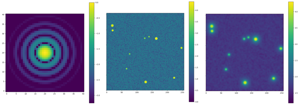
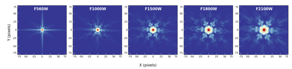
However, many large telescopes these days– including the JWST– are composed of many hexagonal pieces rather than one singular aperture. This changes the shape of the PSF significantly. Compare, for instance, the PSF in Figure 1 to the JWST PSFs in Figure 2; there are quite strong, repeating hexagonal features in JWST’s PSFs, as well as spike features originating from the support structures of additional mirrors. This poses a problem: how do we distinguish sources from the PSF effects? What happens to faint sources that lie in the brightest regions of the artifacts? And what happens to extended sources (like galaxies and nebulae) when convolved with such a PSF? The authors of today’s paper work to remove the effects of JWST’s PSF by deconvolving the image, specifically in the context of active galactic nuclei (AGN), an actively accreting region at the center of some galaxies and which have a variety of both extended features and point source components.
This Work
To figure out how effectively they can deconvolve a JWST image of an AGN, the authors start by building a model image of what they expect the AGN to look like to JWST’s mid-Infrared (MIRI) imaging instrument. This way, they’ll know what the deconvolved image is supposed to look like and can thus better evaluate the performance of the deconvolution methods.
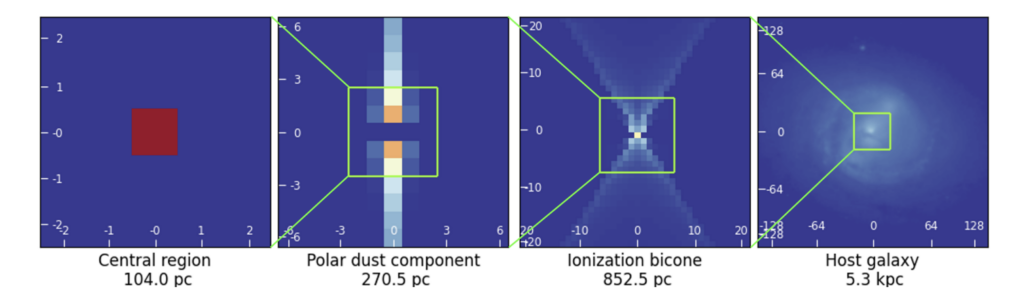
Their AGN model has four components: 1.) the central region of the AGN (panel 1 in Figure 3), 2.) long, collimated outflows of dust originating from the poles of the central region, called polar outflows (panel 2 in Figure 3), 3.) two cones of ionization, called ionization bicones, that are commonly seen in certain types of AGN (panel 3 in Figure 3), and 4.) the host galaxy of the AGN, taken here to be the galaxy NGC 5728 (panel 4 in Figure 3). While the host galaxy and the ionization bicones can be resolved and are thus extended features, the polar outflows can only be resolved along one axis, and the central region appears only as a point source. This makes the model a really rigorous example for the effects of both the PSF and the deconvolution processes.
After building their model to act as a “true” image, they then use it and the JWST PSF to make fake MIRI images for five filters ranging from 5.6 microns to 21 microns. It is this dataset that they use to test five deconvolution methods. Although each method is different, they all work by deconvolving over many iterations until either the size of PSF stops significantly shrinking between iterations or until the difference in flux of a source is different enough from the original image.
Of the five deconvolution methods used, the method that improved the PSF the most– and did so at all wavelengths– was a method called Kraken. Not only did it perform the best in this respect, but it also did it in the fewest number of iterations– 22 iterations at most, while all other methods required between 29 and 105 iterations. Despite the quality of Kraken’s performance, it was not able to make the polar outflow component detectable. Regardless, the method showed true improvement in image quality and so was used to deconvolve a real JWST observation of NGC 5872 that was collected as a part of the Galactic Activity, Torus, and Outflow Survey (GATOS).
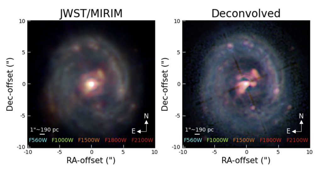
The original JWST image of NGC 5872 and the results of running the Kraken deconvolution method are shown in Figure 4. The Kraken method deconvolved the JWST image both in a similar number of iterations as well as to a similar quality as it had for the mock observation, meaning the results are consistent with expectations! The results also reveal extended structure to the south east of the central region, as shown in Figure 4. Although this feature had been observed in 2019 with other instruments, this feature would be undetectable in JWST images without the deconvolution technique.
Overall, the authors demonstrate the power– and necessity– of deconvolution for doing science with JWST data. It’ll be interesting to see how the deconvolution methods’ performance holds up at shorter wavelengths, as well as to find what other fun features that might have already been missed in previous observations!
Astrobite edited by Isabella Trierweiler
Featured image credit: Made with the WebbPSF Python package and GIMP