Astronomy loves random jargon and simulation work in particular is guilty of this. This Beyond post will go through the basics of numeric simulation jargon with diagrams and examples to help you get moving in astrophysical simulations.
What Are We Even Simulating?
Well, it depends on what you’re working on. If you have a simple two-body problem, you would need those two bodies to know about each other’s gravity in order to produce orbits. This scenario requires the choice of some time step to use to solve kinetic equations (such as F=ma) to update their positions and velocities throughout their orbits.
If you are trying to solve the motion of more than two bodies interacting gravitationally, you would need an N-body simulation. This is more computationally expensive as you have to calculate the interaction between all pairs of bodies, but it is possible to do. Check out this link for an example video of an N-body simulation.
If you have an astrophysical fluid, like a plasma, or something that you can approximate as a fluid, you’ll need to solve the Navier-Stokes equations:
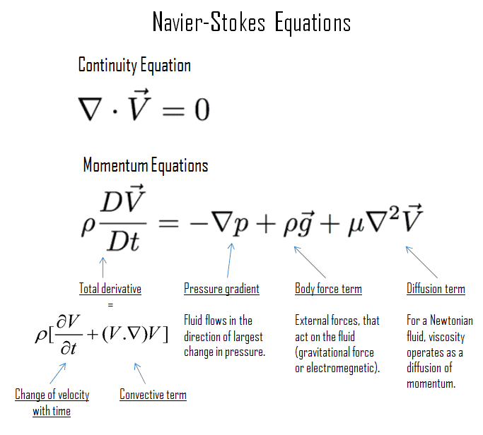
These are partial differential equations, meaning that the calculated progression will always be an approximation, with lots of different choices that will affect how well the approximation works.
If you don’t care about magnetic fields you’ll solve the hydrodynamic version of the equations. If you do, you need the magnetohydrodynamic versions, which require extra care to maintain divergence-free (div dot B = 0) conditions. This is Gauss’ law for magnetism, part of Maxwell’s equations; in our Universe it’s true everywhere but simulations can sometimes end up violating it. Maintaining this condition is usually handled with an extra solver, with every timestep making corrections to fix it.
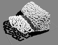
A variant on fluid simulations are smoothed particle hydrodynamics (SPH), which divides the fluid into individual “particles” and then performs gravitational kinetic calculations on each “particle”.
Grids and Coordinate Systems
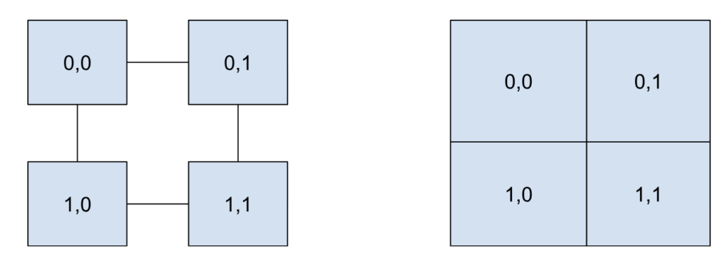
Great, so we have stuff we want to solve. While the Universe is infinite, a computer can only handle a finite region – the domain of the problem. We need to break down or discretize the domain into a mesh of smaller individual chunks. These chunks are usually called cells, and are defined by a set of nodes at the corners and edges or faces that make up the walls. Cells don’t have to be rectangular, although that’s the simplest shape because it’s directly analogous to a matrix, which makes storing all the values super simple. A mesh can either be structured, where all the cells follow a clear geometry of connections, or unstructured, which are more complex to handle in computer memory as they are not analogous to a grid.
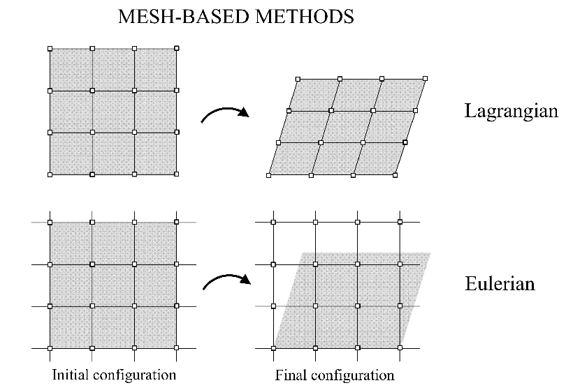
The most common setup is an Eulerian grid, which is a stationary or fixed grid. You have some region, you slap down some grid lines, and then you solve for evolution in time. This is easy to set up and keep track of.
The alternative is a Lagrangian grid, where the cells actually move and/or change shape with the fluid element contained within them. This is useful if you have a fluid that isn’t doing some kind of uniform bulk motion and you might want more cells in certain areas. However, if the fluid has vorticity, or experiences any amount of rotational motion, these cells can actually tangle together and cause the program to crash. This is usually resolved through an Arbitrary Lagrangian Eulerian (ALE) algorithm, which untangles the mesh around the center of the vortex.
In both cases you might have regions of the domain where you would like some extra resolution. Many programs will allow you to have multiple levels of resolution in the same simulation, a feature referred to as mesh refinement (MR). Usually this refinement is done through an algorithm that calculates how much error you’re accumulating on the PDE approximation due to the lack of resolution in a region, but there are ways to select where you want the higher resolution regions to go. This refinement can be static (SMR) where the refined region is defined and kept constant, or adaptive (AMR), which changes based on some condition in the cells. This can be especially useful when simulating systems that cross multiple orders of magnitude, such as astrophysical jets.
Simulations depend on coordinate systems, which turn out to be the usual suspects you’ll find in a physics or math class: Cartesian x-y-z, cylindrical r-theta-z, and spherical r-theta-phi. Cylindrical and spherical coordinate systems are useful if you have an axisymmetric system, where rotation around theta is essentially uniform. This lets you squish 3D simulations into 2D or 1D, which can be an important strategy if you don’t have millions of CPU hours lying around.
Boundary Conditions And Ghost Zones
Space is infinite, but a computer’s memory is finite. Your simulation is going to have edges which will need special treatment so the solver can actually solve things. The conditions at these edges, referred to as boundary conditions, can be defined in various ways.
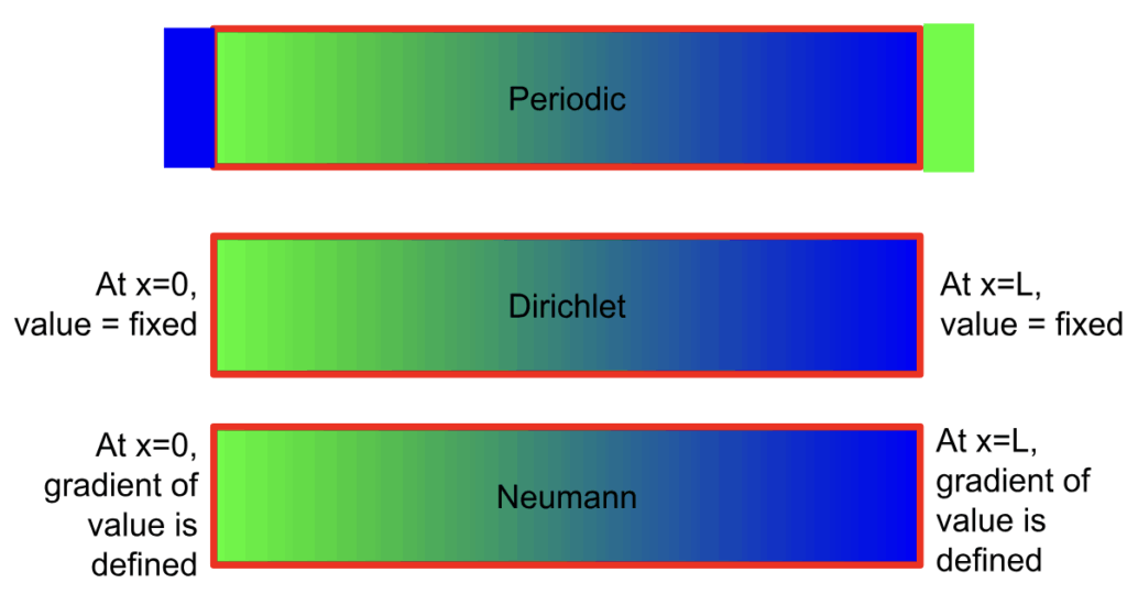
Periodic boundary conditions means that the simulation wraps around each edge. These are often used when there is some sort of periodic wave form in the problem, as it can reveal how quickly the solver is introducing errors.
Dirichlet boundary conditions means that you specified a single value at the edges of the domain. A common problem that uses this is heat transfer through a piece of metal with each end held at a fixed temperature.
Neumann boundary conditions specify the derivative of the function at the edges of the domain. One case would be the dissipation of heat at the surface of a star, for which you could define a constant flux at the boundary. This type of boundary condition relates to some others such as the Robin boundary condition, which is a weighted combo of Dirichlet and Neumann.
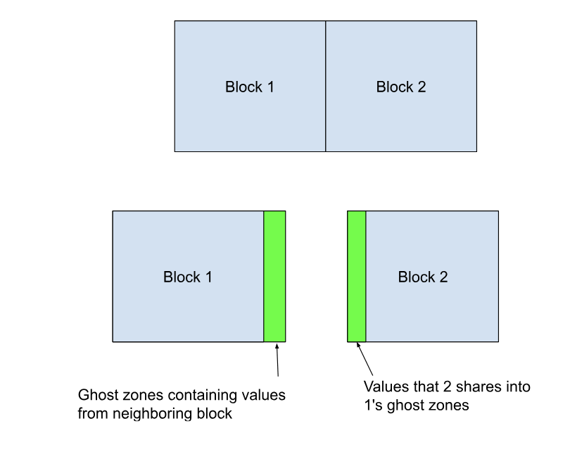
If your simulation is big, the domain is likely split up into multiple subdomains or blocks. Each of these blocks has to communicate what is happening in their section to their neighbors. This is usually done with some extra padding often known as ghost cells or boundary zones. Each block solves for the cells in its region, surrounded by a buffer space. Each block tells its neighbors what’s going on in their borders, filling in the buffer space of adjacent neighbors. This passes information between the blocks and allows them to be solved in parallel, which is vastly preferable to solving the problem in serial. In a perfectly ideal world (which we don’t live in), if you could split a problem into 10 blocks and have 10 CPUs each solve for their own block, you could get a speedup of 10x over having 1 block and 1 CPU. In reality, speedup is less efficient because of the communication required between the blocks, but in many cases a parallel program will beat a serial one.
Simple Solvers
The actual location where the equations are being solved varies between solvers. In a finite difference method, the quantities are calculated at each node. In a finite volume method, the quantities are calculated at the center of each cell.
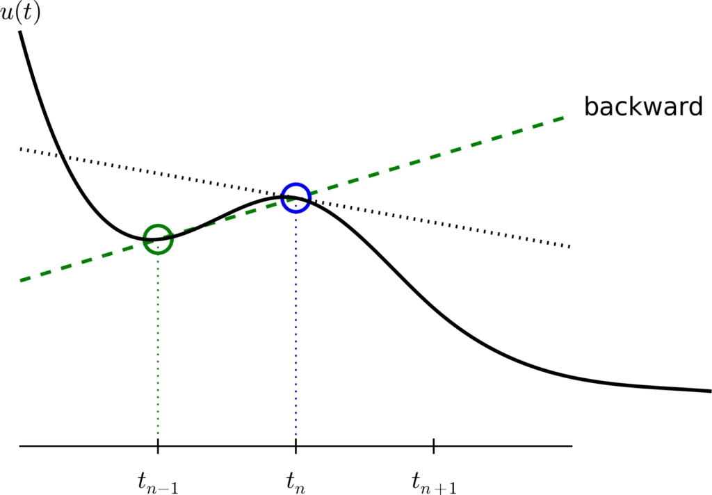
There are two main classes of solvers for differential equations like the Navier Stokes Equations: implicit and explicit methods. In explicit methods, the values of the next time step are determined based on the current time step. The most common version is the Forward Euler Method, where each step is solved as \(y_{n+1} = y_n + \Delta t * \frac{dy}{dt} \vert_{y_n}\). In implicit methods, the values of the next time step are dependent on the future time step. The Implicit Euler method solves \(y_{n+1} = y_n + \Delta t * \frac{dy}{dt} \vert_{y_{n+1}}\).
Other common simple schemes include the Runge-Kutta methods, which takes smaller sub-steps within each time step, and the Crank-Nicolson method, which takes an average of the implicit and explicit results.
Common test cases
Finally, let’s touch on two very common test cases. These tests are useful because they have analytic solutions or known behaviors, which allows for quick comparisons of the stability of the solver you’re using to handle the equations.
The most common is the shock tube, or Sod shock tube test (gif here). In this test, half of the domain is set up with one set of properties, and half with another. The difference leads to a shock forming at the interface between the two regions, followed by the propagation of shock waves throughout the domain.
Another common test is a vorticity test known as the MHD Orszag-Tang test (gif here). Vorticity can be tricky, because Lagrangian meshes can tangle and magnetic fields can lose their divergence free condition. This test produces a spiral vortex, and is useful for evaluating the stability of the MHD shocks that form and interact with each other, and the development of turbulence.
Simulations love their jargon, but hopefully this gave you a quick look at the basics. If you want more, there’s links below to some major simulation codes in astronomy and to some more learning resources to get you going.
Some major codes: Athena++, PLUTO, FLASH-X
Starter Point Resources:
Textbook: Intro to Fluids and Plasmas: An Introduction for Astrophysics [Choudhuri]
Course Notes: Intro to Fluids [UC Berkeley]
CFD Basics: Notes from Cornell Course
Cover Image via Wikimedia Commons
Astrobite edited by Diana Solano-Oropeza