By Briley Lewis
Modern astronomers are often trying to push the limits of what they observe — looking for smaller details, better resolution to observe places like the galactic center and far away exoplanetary systems. One of the key technologies that enables many of these observations (from ground-based telescopes, at least) is adaptive optics. In today’s guide, we’ll be discussing what exactly this revolutionary technology is, and how it works.
What is adaptive optics?
Adaptive optics (AO), broadly speaking, is a kind of technology that corrects for imperfections in a wave of light. It has broad applications, from optometry to astronomy — and for us astronomers, it’s critical to getting diffraction-limited images. This means that instead of angular resolution being limited by the conditions of the atmosphere (the “seeing”), it’s limited by the fundamental physics of light. This angular resolution limit (θ) is related to the wavelength of light you’re observing at (λ), and the diameter of your telescope (D): θ = 1.22λ/D.
Adaptive optics systems detect distortions in the incoming wavefront with some kind of wavefront sensor, compute the needed correction with a control system, and then correct for those distortions, usually with a deformable mirror. We’ll talk more about the technical aspects of AO systems in a bit, but first — we need to think about what’s going on in the images and the atmosphere, so we know what AO is correcting for in the first place.
Understanding your image
The light from a star doesn’t show up in your detector like a perfect singular point of light, due to diffraction. Instead, the light is spread out a bit in a pattern known as a point spread function (PSF). For an ideal telescope with a circular aperture, the PSF is what’s known as an Airy function. This function has a central peak that contains most of the intensity, with rings around that decrease in intensity.
In reality, though, PSFs are often more complicated! The exact PSF depends on the setup of the telescope (e.g. things change if you have a coronagraph, and the new images from JWST show some noticeably funky PSFs!), any imperfections in the optics that make things non-ideal, and the motions of the atmosphere.
There are a few ways we measure a PSF, even when it’s a bit lumpy. The Full Width at Half Maximum (FWHM) measures the size of the PSF, and the Strehl Ratio compares the actual observed intensity of the Airy function’s center to an ideal value: S = Iobs/Iideal where S is always less than 1 (when Iobs = Iideal). The higher the Strehl, the better the image you’ve got!
Some of the distortions in a PSF are known as speckles — blobs of light on the PSF. Quasi-static speckles arise from imperfections in the optics, and are pretty stable over time, whereas atmospheric speckles come from (you guessed it) the atmosphere and change very rapidly. The atmosphere is one of the biggest issues for getting a stable, crisp image, and that’s why we have adaptive optics!
Turbulence & what’s going on in the atmosphere
Next, let’s dig into what’s going on in the atmosphere to create these speckles we have to deal with using AO. The air in Earth’s atmosphere isn’t perfectly uniform — different pockets of air have different temperatures, and correspondingly different indices of refraction. Different temperatures of air mix and interact as well, causing turbulent motion (e.g. what you see on a hot day over asphalt). Light coming from a distant star enters the atmosphere as a flat plane wave, and is then distorted by these variations in the air, known as turbulence.
Caption: Illustration of factors in atmospheric turbulence. Image from James Graham, Berkeley.
Note: For those getting into research into AO, we’re going to get a bit more into detail about atmosphere models. If you don’t want this much detail yet, feel free to skip the next two paragraphs!
The Kolmogorov model is a popular choice to describe turbulence. It describes energy added to the atmosphere (on some outer scale, L0) that is transferred to smaller and smaller variations (with a limit at the inner scale, l0) through turbulent motions. The inner scale is limited by viscosity, which dissipates the turbulence. This model predicts that the turbulence power spectral density (“the turbulence strength at different spatial scales” as described by Claire Max) is ɸ(k) ~ k-11/3 where k is the wavenumber k = 2*pi / λ and λ is the scale of the turbulence. It also predicts something called the phase structure function, which describes the difference in index of refraction (DN) between two points in the atmosphere a certain distance (r) apart: DN(r) = CN2r2/3 where CN2 is known as the structure constant. CN2 describes the strength of the turbulence — larger constant, stronger turbulence!
Another relevant parameter is the atmospheric coherence length, also known as the Fried parameter (r0). The Fried parameter describes how far apart two points on a telescope are for the correlation between them to decrease by a factor of e; essentially, it’s a measure of how correlated the atmospheric turbulence is, and is related to CN2 plus the wavelength of light you’re observing in and the zenith angle (how close to the horizon you’re observing, related to the airmass). If the atmosphere is really turbulent (CN2 is large), then r0 will be small. Conversely, for a more still atmosphere (CN2 is small), then r0 will be large. If r0 is larger than your telescope, then you really don’t even need adaptive optics!
There is another assumption that makes thinking about turbulence a bit easier, too. The pattern of turbulence changes over time, but that’s often pretty slow compared to the wind. An assumption known as Taylor frozen flow states that the turbulence seen by a telescope at a given time can be described as the turbulence at an earlier time shifted a distance based on the wind velocity.
Turbulence & what’s going on in the atmosphere
Next, let’s dig into what’s going on in the atmosphere to create these speckles we have to deal with using AO. The air in Earth’s atmosphere isn’t perfectly uniform — different pockets of air have different temperatures, and correspondingly different indices of refraction. Different temperatures of air mix and interact as well, causing turbulent motion (e.g. what you see on a hot day over asphalt). Light coming from a distant star enters the atmosphere as a flat plane wave, and is then distorted by these variations in the air, known as turbulence.
Note: For those getting into research into AO, we’re going to get a bit more into detail about atmosphere models. If you don’t want this much detail yet, feel free to skip the next two paragraphs.
There is another assumption that makes thinking about turbulence a bit easier, too. The pattern of turbulence changes over time, but that’s often pretty slow compared to the wind. An assumption known as Taylor frozen flow states that the turbulence seen by a telescope at a given time can be described as the turbulence at an earlier time shifted a distance based on the wind velocity.
In reality, the atmosphere also has multiple layers — something that can make simulations a bit more complicated! The wind speed and turbulence can be quite different at different heights. A few layers of note are the planetary boundary layer and the shear zones. The planetary boundary layer is near the ground (up to a few kilometers), and often has the strongest turbulence. The shear zones, on the other hand, are much higher up (around 10-20 kilometers) and have strong winds, like the jet streams.
So, why do we care so much about the atmosphere? Well, because it’s directly related to what we see through the telescope! The view of the pupil plane (e.g. where the light enters the telescope) shows the atmospheric turbulence, and that is related to the image we observe in the focal plane with our detectors by Fourier transforms. Fourier optics is a bit beyond what we’ll cover in today’s bite, but it’s super relevant for AO and for anyone interested in instrumentation — check out the references at the end of this article for more info.
Wavefront sensing and control: how we detect and correct distortions from turbulence
Some adaptive optics systems sense the light from the star you’re observing (or a nearby one), known as Natural Guide Star adaptive optics (NGAO). Others use a laser to create an artificial star, known as Laser Guide Star adaptive optics (LGAO), like the famous Keck telescopes used as the cover image for this Astrobite. Either way, there is a detector (the wavefront sensor, WFS) that will observe the incoming light from the guide star.
Two of the most popular wavefront sensors are the Shack-Hartmann WFS and the Pyramid WFS, both illustrated in a figure below. The Shack-Hartmann WFS uses a series of small lenses known as lenslets to create images from across the pupil plane (known as subapertures). These images are displaced from a perfect grid by distortions, and their displacements can be used to calculate the distortions so we can correct them. The Pyramid WFS uses a four-sided pyramid instead of lenselets, splitting the light into four images. Differences between those four images can be used to calculate distortions.
One useful way to represent the different distortions in the wavefront is the set of Zernike polynomials. These show optical effects like tip, tilt, focus, astigmatism, and coma. These are used to represent the wavefront errors from a circular telescope mathematically, and we can think about “removing” each of these Zernike modes to correct our image.
After the wavefront is determined, there needs to be a way to correct for the distortions. This is where deformable mirrors (DMs) come in! DMs are exactly what they sound like — mirrors that can change shape to reflect the light from the distorted wavefront, and hopefully correct for the distortions. There are many different types of DMs, such as piezoelectric mirrors, which have small actuators that push on a thin glass mirror to change its shape, and MEMS (microelectromechanical systems) mirrors, which are on silicon chips.
Corrections can be applied with an open- or closed-loop control system. In an open-loop system, the light comes to the WFS before the DM, so you can’t check how good the correction was or integrate that feedback into a new correction. In a closed-loop system, the light hits the DM first before going to the WFS, so a feedback loop is created to continually improve the wavefront correction.
Although we can do pretty well with our corrections, there are multiple errors to consider. DM fitting error arises because we can only make actuators so small, so we can’t perfectly fit the wavefront distortion. Servo lag error comes from the fact that our motors driving this whole mechanical process can only move so fast — there is a finite amount of time needed to measure and correct the wavefront. Another is non-common-path errors, which happen because the light going to the detector and the light going through the AO system aren’t the same, so they encounter different errors in the optics. Plus, we’ve always got the typical read noise and photon noise, which we count as wavefront sensor measurement error.
There’s also something called isoplanatic error or anisoplanatism, which arises when the patch of sky where the guide star is has different turbulence than the patch of sky where you’re observing. Guide stars are often chosen to be very close to the science target to avoid this issue.
What comes next for adaptive optics
Researchers are working constantly to improve our AO systems, including limiting or addressing all these sources of error. Here’s a short list of some of these ongoing areas of research:
- Multiconjugate AO — the idea of using multiple WFS and DMs together to make the correction even better
- Predictive control — using information about wind speed, prior corrections, etc. to change the correction and account for changes that happen between the WFS and DM. No need to worry about fast response times if you can predict the correction!
- Focal plane wavefront sensing — instead of putting a WFS at the pupil plane, what if you put it at the focal plane so it could correct the exact same light path, avoiding non-common path errors?
- Sensor fusion — the idea of using information from many sensors, not just the DM, to improve the wavefront correction. Very related to predictive control!
- Ground layer AO — adaptive optics systems specifically to address the really turbulent lower layer of the atmosphere
- AO for ELTs — with the upcoming extremely large telescopes (TMT, GMT, E-ELT), we need to figure out how to make scaled-up adaptive optics!
If you’re interested in learning more about adaptive optics, check out the resources below and look into the Center for Adaptive Optics AO Summer School!
Astrobite edited by: Pratik Gandhi, Lili Alderson
Featured image credit: Keck Observatory
Some examples of AO systems (definitely non-exhaustive!):
- TMT’s many planned AO systems (NFIRAOS, MIRAO, MOAO, ExAO, GLAO)
- Keck’s AO system
- Subaru SCExAO
- UC Lick Observatory AO
- VLT AOF
- Palomar PALM-3000/P3K
Some relevant Astrobites:
- It’s a Bird, It’s a Planet, It’s a….Speckle?
- Optics to outrace them all
- Zooming in on Betelgeuse
- Star formation in the galactic center
- The birth of a baby planet
- How do you see a firefly next to a spotlight?
- Is this how we’ll discover missing black holes?
- The Nobel Prize in Physics 2020: Andrea Ghez
- Young, massive, and mysterious
- First photos of a baby planet
- H0ly cow! A new measurement of the Hubble constant
Resources:
- Fundamentals of Atmospheric and Adaptive Optics by Paul Hickson (2008)
- Adaptive Optics Tutorial at CTIO
- Annual Reviews: Extreme Adaptive Optics by Olivier Guyon (2018)
- CfAO Summer School
- Adaptive Optics for Astronomical Telescopes by John W Hardy
- Claire Max Intro to Adaptive Optics
- A Tour of AO Systems Worldwide
- The Fourier Transform and Its Applications by Bracewell
- Intro to Fourier Optics (Goodman)
- A Student’s Guide to Fourier Transforms (James)


JWST PSF link-rot: https://www.stsci.edu/jwst/science-planning/proposal-planning-toolbox/psf-simulation-tool
Literally sister this type blogs or educational articles are absolutely outstanding and essential for everyone!
Thank you so much for sharing these types of amazing knowledge with us ❤️
Best explanation I have ever seen!
Clear and wonderful explanation, thanks a lot!