Authors: S. Kiefer, A. J. Bohn, S. P. Quanz , M. Kenworthy, and T. Stolker
First Author’s Institution: Institute for Particle Physics and Astrophysics, ETH Zurich, Wolfgang-Pauli-Strasse 27, 8093 Zurich, Switzerland
Status: Accepted to A&A Journals [open access]
The background
A huge amount of effort goes into designing and manufacturing high-quality telescopes and instrumentation so that astronomers can have the best possible data. Then a similar Herculean effort goes into analyzing this data and understanding the underlying physics of the phenomena observed.
A third layer of brilliance also exists: this is the range of ingenious observational techniques and tricks employed by astronomers and telescope operators to gather data. These vary across wavebands and allow us to push the capability of the hardware beyond its typical limits.
Examples of such work include the combining of different telescopes to simulate one large telescope (e.g. the EHT) or the use of clever adaptive optics (AO) techniques to squeeze out some more performance percentage points.
The techniques described by the authors of today’s paper, used to directly image exoplanets, are collectively known as differential imaging. The direct imaging of exoplanets, due to the proximity to their relatively bright host stars, is often compared to trying to see a firefly next to a spotlight. The bright source, and the resulting speckles from the atmospheric turbulence, dominate the signal in the vicinity of the star.
So how does this work? There are quite a few new acronyms in the next section, but bear with me!
The method
There are two key types of differential imaging, both described nicely in the context of SPHERE here:
- Angular differential imaging (ADI):
- ADI works by turning off the instrument derotator, a device usually used to compensate for the rotation of the earth. This causes the field of view (FOV) to rotate around the target star during observations.
- Therefore a potential exoplanet rotates around the stellar position during the observation. The images can be used to build a model of the stellar PSF with negligible contribution from the companion, which can then be subtracted from each individual image. Also discussed in a previous astrobite.
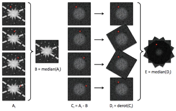
Figure 1 – Diagram explaining how the Angular Differential Imaging technique works.
- Spectral differential imaging (SDI):
- The general principle of SDI is that two images of the star acquired simultaneously at close wavelengths can be subtracted to remove most of the stellar halo and speckle pattern. In fact speckles are located at an angular distance from the star in proportion to their wavelength.
- If images are taken at wavelengths very close together, so the PSF is as similar as possible in the two images, and the two images are also taken simultaneously, in order to avoid that the speckle pattern will change from one to the next, and they are radially scaled to a common wavelength, then the difference of images should cause the fixed-pattern speckles to drop out.
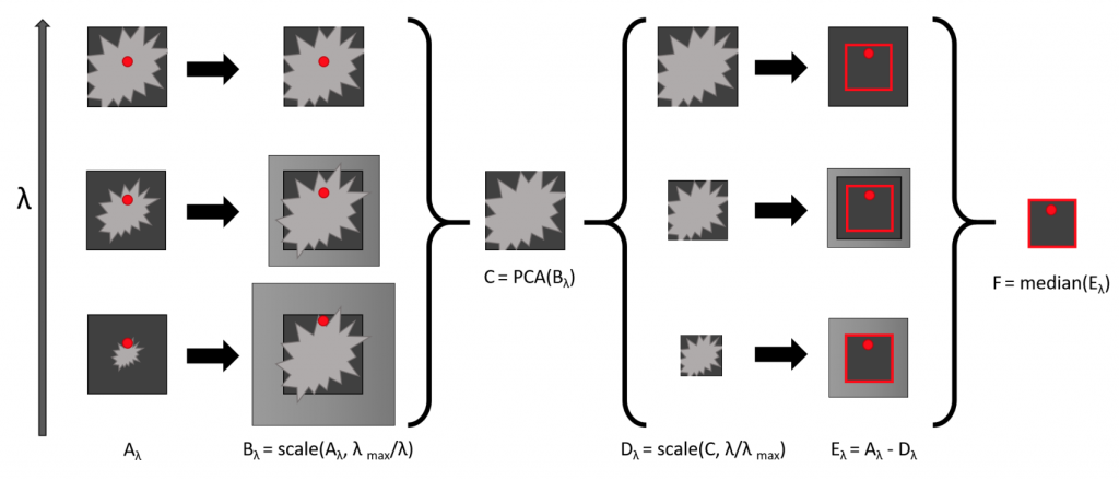
Figure 2: Spectral Differential Imaging
Kiefer et al. use both of these techniques and also explore the use of three different combinations of ADI and SDI. They also utilise a mathematical technique called Principal Component Analysis (PCA), a nice visual explanation of which can be found here. The three combinations of ADI and SDI are:
- Combined Differential Imaging or CODI: First, all images are scaled according to λ using a scaling factor S (λ) = λmax/λ. Afterwards, a PSF model is created using PCA. The PSF model is then subtracted from each image. Lastly, all images are scaled back before they are derotated and stacked using the median in order to create the final image.
- SADI: First SDI is performed as described above but without derotating and stacking after the reduction. Afterwards it performs ADI as described above to create the final image.
- ASDI: First ADI is performed as described above but without derotating and stacking after the reduction. Afterwards it performs SDI as described above to create the final image.
So what were the results?
It might not surprise you that the different combinations of ADI and SDI generally outperformed the basic techniques on their own.
The large range of results in the paper are complex and include analysis on the signal to noise ratio (S/N), noise components, model completeness, dependencies etc., so I have picked out a few key plots based on the S/N to illustrate the general performance differences.
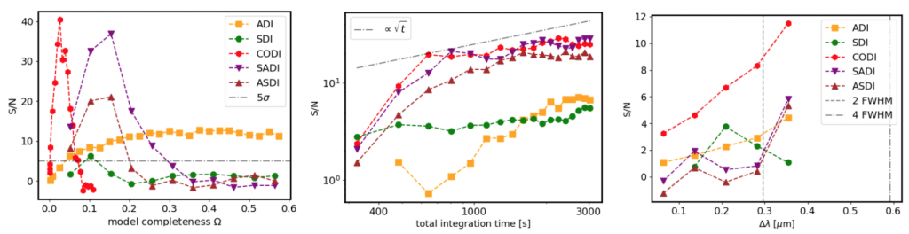
Figure 3: Key S/N results from the paper (hint: high S/N is good!)
For the targets under test, using a combination of ADI and SDI consistently achieved better results than using ADI alone. SADI and ASDI performed similarly but target-specific differences can occur. In all tests, CODI achieved the highest S/N and constantly performed slightly better than SADI or ASDI.
Throughout the paper they reference their use of the Python package PynPoint, so if you’re a Pythonista and want to learn more about these techniques follow the link!
Astrobite edited by Luna Zagorac
Featured image credit: ESO
Author