One of the coolest parts of doing research is that your work is right on the cutting edge of what’s known. At the same time, this can be one of the toughest parts, as some of the most interesting signals are the ones buried deepest in the noise. As a result, the careful observational astronomer moonlights (daylights?) as a statistician. Understanding your sources of noise well and dealing with them appropriately is necessary to ensure that you neither overstate your results nor miss out on exciting discoveries. Today let’s talk about noise, how to deal with it, and what to do when your noise isn’t as simple as you might want.
Let’s say we have some data. Maybe it’s a spectrum, maybe it’s time series photometry. For this scenario, let’s say we have n measurements of some parameter and that we know each xi value for our data (frequencies, times) very precisely (here, the i subscript refers to an individual measurement). We also know the measurement values (the yi at each xi), and have a good idea of the uncertainty (σi) associated with each data point. If we want to find the best-fitting model to these observations*, then the standard practice is to evaluate the model at our data points, measure the residual (ri) between our data and the model, and then calculate a χ2 value by evaluating the sum of (ri /σi)2. The model that minimizes this value is our best-fitting model.
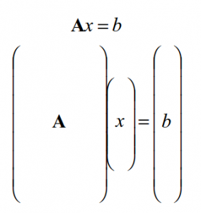
But what are we really doing here? While it may not be evident from the math above, the calculation of χ2 has its roots in matrix manipulation. In fact, we can show through a few matrix operations why χ2 works for finding the best fit to a system of equations. You may have seen this before if you have taken a linear algebra course! If our model is linear, then we can write that b = Ax, where A is a set of linear equations, b our measurements and x our model parameters. We then have a matrix that looks like this:
You might remember from your linear algebra course that, to find the best-fitting value for x, we want to minimize (b–Ax)T(b–Ax). (If you don’t remember this, you don’t have to take my word for it: check out this pdf for a quick refresher.) In the case where each value of b also has a known uncertainty, then we instead want to minimize (b–Ax)TC-1(b–Ax), where C is a diagonal matrix, with the squares of the individual uncertainties (the variances) along the diagonal.
That looks like a lot of math. But in this case, (b–Ax) is our residual vector! To simplify our lives, let’s call it r. In this case, the value we want to minimize is (r)TC-1(r) ≡ ∑ (ri /σi)2. This is exactly chi-squared! Evaluating χ2 is, in this case, identical to performing these matrix operations.
There’s one assumption we’ve made throughout which makes the matrix math identical to evaluating chi-squared: we assumed that when we collected our data, the individual yi observations were independent. That is, each yi depends only on its xi, and not on other values of yi. This is often a reasonable assumption, but not always! For example, a light curve of a star might contain contain correlated noise caused by the star’s rotation or stellar activity. Quasar light curves also might contain correlated noise due to slow changes in the accretion rate of the central black hole. Sometimes, the correlated noise isn’t astrophysical, but instrumental: observations from Spitzer, for example, often contain correlated noise as the spacecraft moves slightly over the course of an observation.
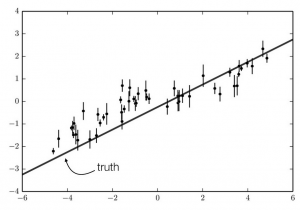
Our simulated observations. The data are drawn from a model that is a straight line (shown on the plot) with correlated noise included.
Correlated noise can significantly affect our results if not properly accounted for. In general, correlated noise causes our error bars to be underestimated. This makes sense! To understand why, let’s look at some real (fake) data. Here, I created some data by randomly drawing from a model that has a positive slope and adding correlated noise. The data are shown in the figure to the left.
If our noise is uncorrelated, and a few consecutive data points are all significantly above our model (like around x=-1 in our example), then they will all contribute to a calculation of a large value for χ2. In this case, a model that provides a larger value near x=-1 will be heavily favored over the “truth.” Really, these points are above our model because all the other points around them are above our model. Therefore, χ2 is insufficient to fully describe our observations. Because yi and yi+1 depend on each other (as well as yi-1, yi+2, and all the other nearby data points), each residual should be trusted less than the full ri /σi weight we discussed above.
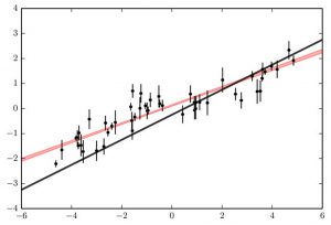
Same as the previous figure, with the 1-sigma range for the best-fitting line to the data shown in red. Clearly, the correlated noise has caused us to underestimate our uncertainties.
To see this graphically, let’s try to fit these fake observations to a straight line. In our fitting, let’s treat the observations as if they were perfectly uncorrelated, and attempt to minimize χ2. The result of this fit is shown in the figure to the right. The red shaded region shows our 1σ range on the line that describes our data. As we predicted, the model predicts a significantly larger value near x=-1 than the truth. In this case, we have a very tight measurement of what the slope of the line that describes our data should be. We would expect that if the shaded region were representative of the actual acceptable range of parameters that fit our data, that the truth (our black line) would be included in the shaded region. Unfortunately, the constraints do not match reality at all, as only significantly shallower slopes than the truth are predicted. In this case, not accounting for correlated noise means we have the wrong answer! It also means that we think we did a great job in our measurements. We have very small error bars in our fit; the red shaded region is very narrow, so we think the region in which the truth could lie is tightly constrained.
Luckily, there are techniques to account for correlated noise. To do this correctly, we need to leave behind our simple chi-square calculation and use the power of C. Not the ocean, but our uncertainty matrix from earlier! Before, we said if our noise is perfectly uncorrelated, or white, then χ2 is mathematically the same as evaluating (r)TC-1(r). C‘s official name is the “covariance matrix.” Each element in the covariance matrix shows the relation between two observations yi and yj . If the two observations depend strongly on each other, Cij is relatively large; if the two observations have no dependence on each other, Cij is zero. If the two observations are the same (i=j), then Cii is the variance σi2.
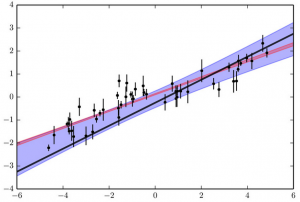
Same as the previous figures, with the 1-sigma range for the best-fitting line to the data when correlated noise is accounted for shown in blue. Only by accounting for correlated noise do we find a model that without an overstated precision.
Therefore, by modifying the covariance matrix C and solving (r)TC-1(r) instead of just summing (ri /σi)2, we can account for correlated noise in our model. In the figure to the left, I’ve modified my uncertainty calculation to account for my updated covariance matrix, and again attempted to find the best-fitting line to these fake data. The region of acceptable values is shown in blue. This time, we find that the truth is included in our 1σ uncertainties! Our error bars are larger, but these are physically meaningful: the original error bars (in red) didn’t accurately describe the uncertainty in our model, while these do. With this fit, we can be satisfied that we have the most accurate result the data can provide.
Of course, in this example I knew what my correlated noise should be, and was able to modify C to exactly represent this noise model. In the real world, we don’t always know exactly what our noise model should be, so we don’t know exactly what C should look like. This makes the problem more difficult, but not intractable! There are two primary techniques used to treat correlated noise in real life:
1) Estimate C with some other data, and use this covariance matrix instead of a perfectly diagonal one. This is useful when you have plenty of data from which a reasonable estimate of C can be drawn. An example of this might be Kepler data, when looking at planet transits. The transit of an Earth-like planet occurs once per year, for 13 hours, leaving 364.75 days of stellar and instrumental noise between each transit. This data can be used to probe the noise and its correlations for the star in question, which can then be applied to each transit event.
2) Assume a functional form of C and allow the parameters that define this function to vary. Maybe you know that a certain point is going to be influenced by points that are very close to it only. Maybe you’re looking at a rotating star and you know the noise is going to be correlated with noise exactly one stellar rotation period apart. In these cases, you can define C as a function of a few other parameters and fit these parameters at the same time as you fit your astrophysical model. The benefit of this technique is that you can constrain the correlation in your noise, as long as the function that you have assumed is representative of the true noise in your data! This technique is the basis of Gaussian processes, a popular technique for dealing with correlated noise in data.
Correlated noise can be tricky, but it doesn’t have to be scary! There are existing techniques to deal with it, and even packages to make these techniques accessible to newcomers. Understanding when to go beyond χ2 is necessary to ensure that your uncertainties are correctly estimated; techniques like the ones above should be a part of any observational astronomer’s toolkit.
The author would like to thank Dan Foreman-Mackey (NYU) for use of the figures in this post.
*Here, I’m assuming we know what the functional form of the model should be. Model selection is an entirely different topic, and could be the topic of a separate blog post/textbook.



Fantastic post that really breaks down the problem. Follow-up question for you. What if you have highly correlated data with unknown covariance (a great candidate for Gaussian Process regression) yet you still need to fit a parametric model to your data (because you have some physical model to explain it)? In that case, fitting the GP is only half the battle. You need to find a parametric model that matches your GP as closely as possible. I haven’t been able to find ANY literature on how to compare some arbitrary parametric density to a GP – do you have any thoughts or resources on that?
Thanks!
Hi Charles,
I might be misinterpreting your question—I think you’re saying you want to use a GP noise model and simultaneously fit a model to the data? In this case, I would fit a model, calculate the residuals between the model and the data (simply by subtracting one from the other) and then measure your likelihood by fitting your GP model to the residuals. You can then do error estimation by seeing how your likelihood changes as you either vary your (parameterized) data model or your (flexible GP) noise model, maybe inside an MCMC scheme, and see how covariant your model is with your noise. Or you could figure out the overall uncertainty in your model by then marginalizing over all the GP noise parameters.
Does that answer your question?
“you want to use a GP noise model and simultaneously fit a model to the data”
Yep, that’s exactly it! I’m surprised it’s not a more common problem, actually. I have to explain my data using a parametric model – in my case, particle coordinates (each produces a spherical signal). But my data, like the what you describe in your post, has locally correlated errors due to instrumentation and processing. The way we consider data error is critical in evaluating model likelihood: assuming all data points are totally independent gives a much higher “data weight” than if there is some correlation. The way I think about it, when there’s more data covariance, it’s like you have a smaller data set with fewer points to satisfy. If that makes any sense!
Your suggestion of fitting a GP to the residuals is very compelling. Say I do the fit, and in the process I estimate residual covariance. I suppose I could use it to evaluate the model likelihood by using it as the covariance function of a multivariate normal, or:
L = Normal(residual vector | 0, GP_covar).
That would involve inverting a huge matrix (the data can have millions of voxels) but it’s a promising idea. Assuming I understand your suggestion correctly! Thanks for your help.
Okay cool. I think we’re on the same page.
It does involve doing costly operations on a huge matrix, and that’s usually the biggest computational part of using a GP method like this! You can make some assumptions sometimes that may be physically warranted in this case to speed up the computation. Maybe each data point is correlated with points very close to it, but is (very nearly) uncorrelated with points far away. In that case you could assume the well-off-diagonal elements in your covariance matrix are zero, and you have a banded matrix, which is relatively more efficient to solve. More generally, if you can make an argument that any points aren’t covariant with specific other points, you can make those covariance terms exactly zero and find yourself dealing with a sparse matrix (one that’s mostly zeros) which is much more efficient.
If you do have some covariance between each point and *every* other point, then you’re probably just going to have to suck it up and do slow matrix operations. It’s a bummer, but it’s the price of modeling things correctly!
why not do your estimations using Non-Parametric Regression? It is ALOT more computationally less expensive than parametric models, however more complicated to code.
Hi Ben, I’m probably chancing it hoping I can pick your brain on this subject 3-4 years after the post date. But let’s try. I’m trying to get my head around one issue with the covariance matrix in this equation. When inversing C some of its values become negative, what causes that the final chi^2 may be negative – chi^2 is a one sided test, so what am I doing wrong here?
To give more specific details for my particular problem I’m trying to solve: I have a bunch of data, but only some of the data points are correlated. I know how to parametrise the correlation (though I still have to solve for one parameter there, which just simply causes there is one additional free parameter in the chi^2 minimisation). So with the knowledge of which data points are correlated and how to parametrise the correlation I coded an appropriate covariance matrix. But then inverting the matrix in the minimisation equation causes negative values and in return may cause negative chi^2. Any suggestions are welcome!