Title: A systematic search for transiting planets in the K2 data
Authors: Daniel Foreman-Mackey et al.
First Author’s Institution: New York University
In May 2013, the Kepler mission came to an end with the failure of a critical reaction wheel. This reaction wheel was one of four that was responsible for keeping Kepler focused on a fixed field of view so that it could perform its mission: to continuously monitor the brightness of the same 150,000 stars, in order to detect the periodic dimming caused by extrasolar planets crossing in front of their host star.
A year later, in May 2014, NASA announced the approval of the K2 “Second Light” proposal, a follow-up to the primary mission (described in Astrobites before: here, here), allowing Kepler to observe —although in a crippled state— a dozen fields, each for around 80 days at a time, extending the lifetime of humanity’s most prolific planet hunter.
The degraded stabilization system induces, however, severe pointing variations; the spacecraft does not stay locked-on target as well as it could previously. This leads to increased systematic drifts and thus larger uncertainties in the measured stellar brightnesses, degrading the transit-detection precision — especially problematic for traditional Kepler analysis techniques. The authors of today’s paper present a new analysis technique for the K2 data-set, a technique specifically designed to be insensitive to Kepler’s current pointing variations.

Fig 1: The K2 mission is Kepler’s second chance to get back into the planet-hunting game. Kepler’s pointing precision has however degraded, but novel pointing-insensitive analysis techniques aim to make up for that. Image credit: NASA/JPL.
Traditional Kepler Analysis Techniques
Most of the previous analysis techniques developed for the original Kepler mission included a “de-trending” or a “correction” step —where long-term systematic trends are removed from a star’s light curve— before the search for a transiting planet even begins. Examples of light-curves are shown in Figure 2. Foreman-Mackey et al. argue that such a step is statistically dangerous: “de-trending” is prone to over-fitting. Over-fitting generally reduces the amplitude of true exoplanet signals, making their transits appear shallower — smaller planets might be lost in the noise. In other words, de-trending might be throwing away precious transits, and real planets might be missed in the “correction” step!
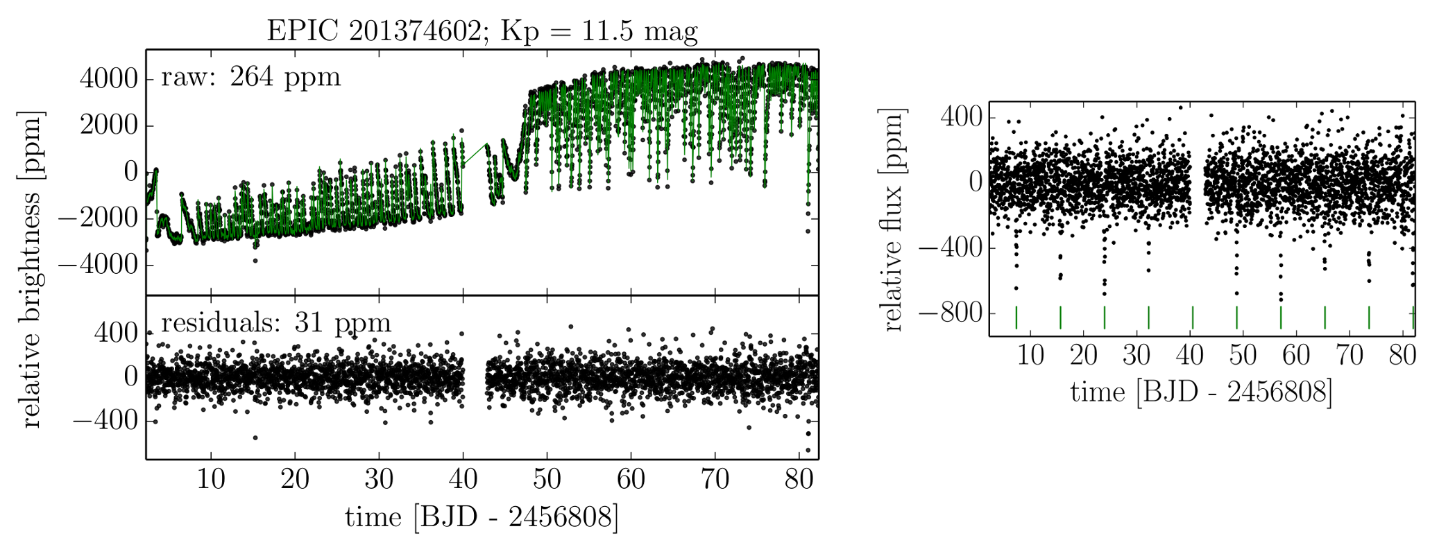
Fig 2: Upper left panel: An illustration of the maximum likelihood fit (green lines) to a K2 light-curve (black dots) obtained from the authors’ new data-driven model. Bottom left panel: The residual scatter i.e. the “de-trended” light-curve, for a given star in the K2 field. The residuals are very small, indicating a good fit. The right panel shows a de-trended light-curve for another star (EPIC 201613023) where the transit events are more evident (marked with green vertical lines). De-trended light-curves like the one on the right were commonly used with past analysis techniques. Foreman-Mackey’s et al. method, however, never uses de-trended light-curves in the search for transits, only for qualitative visualization and hand-vetting purposes (see further description of their method below). Figures 2 (left), and 4 (right) from the paper.
A new analysis method
In light of these issues, the authors therefore sat down to revise the traditional analysis process. They propose a new method that simultaneously fits for a) the transit signals and b) systematic trends, at the same time, effectively bypassing the “de-trending” step.
Their transit model is a rigid model that models each transit to have a specific phase, period and duration. On the other hand, their method to model the systematic trends is much more flexible than the rigid parametrization for the transits. The authors assume that the dominant source of light-curve systematics is due to Kepler’s pointing variability. There are other factors that play a role too, like stellar variability, and detector thermal variations, but the authors focus specifically on modelling the spacecraft-induced pointing variability.
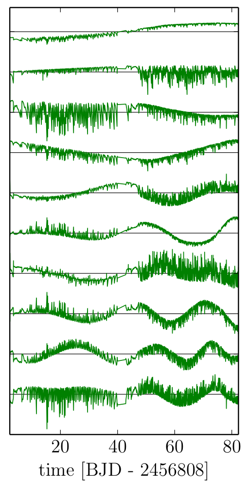
Fig 3: An illustration of the top 10 basis light-curves. A set of 150 make up the authors’ linear data-driven analysis technique. Having a linear model has enormous computational advantages.
Equipped with large amounts of computer power, Foreman-Mackey et al. create a flexible systematics model, consisting of a set of 150 linearly independent basis light-curves (see Figure 3). These are essentially a set of light-curves that one can add together—with different amplitudes and signs— to effectively recreate any observed light-curve in the K2 data-set. The basis light-curves themselves are found by a statistical method called Principal Component Analysis (PCA) —a method to find linearly uncorrelated variables that describe an observed data-set— which will not be described further in this astrobite, but the interested reader can read more here. The choice to model the systematics linearly has enormous computational advantages, as the computations reduce to using familiar linear algebra techniques. The authors note that the choice to use exactly 150 of them was not strictly optimized, but that number allowed for enough model-flexibility to effectively model the non-linear pointing-systematics, while keeping computational-costs reasonable.
With a set of basis light-curves the analysis pipeline then proceeds to systematically evaluate how well the joint transit-and-systematics model describes, and finds transits, in the raw light-curves (see again Figure 2). Finally, the pipeline returns the signals that have passed the systematic cuts: light-curves with the highest probability of having transits.
Results, Performance & Evaluation
The authors apply their analysis pipeline to the full K2 Campaign 1 data-set (including 21,703 light-curves, all publicly available here). The systematic vetting step returned 741 signals, which were further manually hand-vetted by the authors; throwing out, for example, obvious eclipsing binaries. The authors end with a list of 36 planet candidates transiting 31 stars —effectively multiplying the current known yield from K2 by a factor of five! Figure 4 (left) summarizes the distribution of the reported candidates in the radius-period plane.
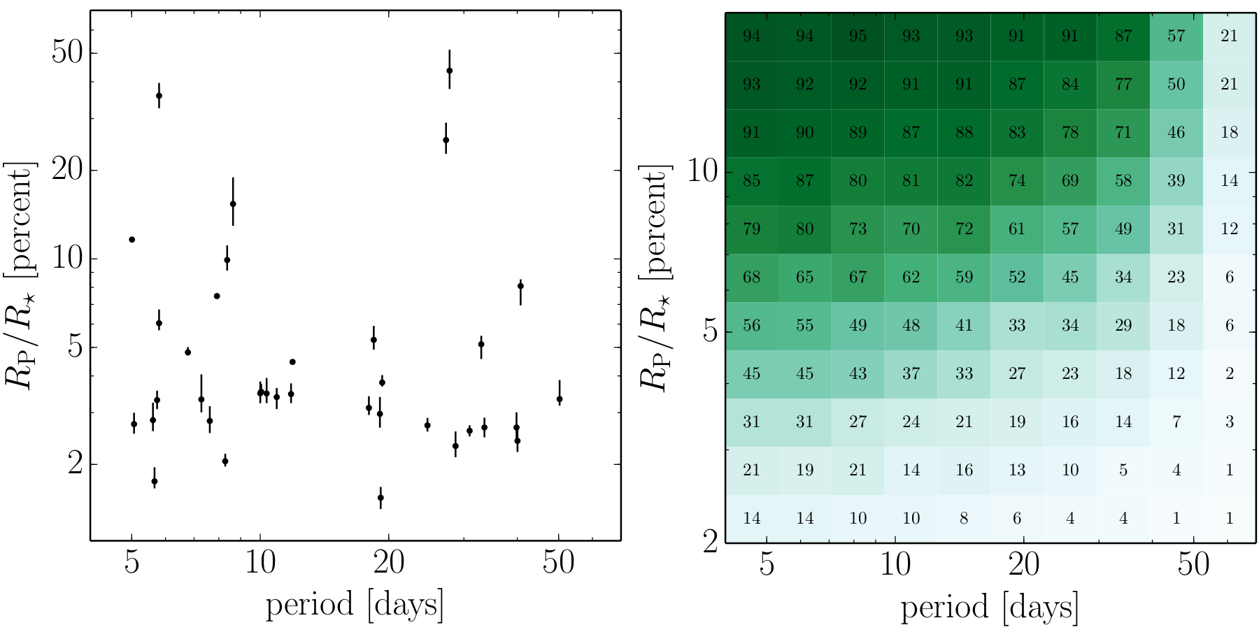
Fig 4: Left: The fractional radii of the reported 36 planet candidates as a function of their period. Right: Detection efficiency in the radius-period plane, calculated by injecting synthetic transit signals into real K2 light curves, and calculating the fraction that are successfully recovered. Figures 11 (left) and 9 (right) from the paper.
The authors also discuss the performance and detection efficiency of their method. By injecting synthetic transit signals into real K2 light curves and measuring the fraction that are correctly identified and recovered by their pipeline, gives an estimate of the expected performance under real analysis conditions. From Figure 4 (right) we see that their analysis technique performs the best for short-period large-radius planets. This makes sense: larger planets have larger transit signals, and shorter orbital periods increase the number of observed transits; they are more probable to be successfully found.
Lastly, the authors share their data products online, along with their pipeline implementation under the MIT open-source software license. This means that anyone can take a stab at reproducing their findings, or perhaps even find new transits signals! So, now I want to ask you, dear reader, will you lengthen the list of known planet candidates today?
Author
Did using linear models for computational reasons seem to impact the analysis/conclusions much? Could some other nonlinear model possible have found other possible transits, or was this model actually too liberal (since it seems like the authors had to rule out a large percent of the possible transits the study initially identified)?
The usage of linear models impacted the analysis/conclusions in that we were able to have them! We first started out playing around with more sophisticated ideals (modeling everything that comes into the system properly) using a pretty sweet optimizer called ceres. It’s the same one Google Maps uses to optimize your route. It turns out the problem was completely intractable with the processing power we had, so we had to descope. We’re thinking about the right ways to add in complexity.
This sounds like a great method to get around flaws in the data, and it seems to be pretty effective. I look forward to the new discoveries that come out of using this method.
Same here Jennifer !
This seems very similar to another paper I read in that they inserted a set of false positives (eclipsing binaries) in order to deduce true planet signals. Interesting read! I wonder if they will ever launch a mission to repair Kepler like they did for Hubble…
Unfortunately no. Kepler isn’t in low earth orbit like Hubble, it’s in an Earth-trailing orbit, moving slowly away from us. This is a good thing for planet finding, because it means Earth never gets in your way and you can always observe the same region of space (as long as you choose your region smartly!) but a bad thing for service missions, because it’s now about 1 AU away.
This looks like a great way to keep Kepler running! Do you know how long it will remain operational using these techniques?
Hi Chris! It surely is an exciting technique, and shows some very promising results when used on the K2 data, but it will also be interesting to see what the technique can dig up when applied on the original Kepler data. For now, the K2 mission is designed to extend the lifetime of Kepler for 2-3 more years — assuming of course that the last 2 reaction wheels keep working!
I wonder if this new method could be as effective on the original Kepler data analyzed using traditional means. From the outline of this article, it seems possible that planets lost in the de-trending process could reappear using a new modeling process.
Yeah, that’s the idea! Dan originally wrote this code to find small, Earth like planets on 1-AU like orbits in Kepler data. We then decided to apply it to these data because it was a similar problem. But the intention has always been for Dan to use it for Kepler data!
When space-based telescopes break, how often are we able to salvage them using techniques like this? How often are we able to salvage them by physically repairing them?
Good question Anne! Like every piece of technology, scientific instruments have a limited life-time — and fixing them physically is usually a matter of cost (— and going to space is expensive!) We have been able to fix/upgrade the Hubble space telescope because it is in relatively close orbit (Earth orbit at ~550km), but fixing Kepler was deemed unfeasible as it is so far away from us (Earth-trailing orbit ~140,000,000 km!) Sometimes we can make well-informed corrections to the data, like in the case of Kepler. Other times, things are more tricky, and there is little that we can do in software, and physical corrections to the instrument are necessary.
Given that those planets are so far away from us, are we ever going to know more about them than their existence and physical characteristics?
Oh sure. We’ve characterized atmospheres of planets, their interior structures, how cloudy they are… upcoming missions like JWST may be able to infer the presence of water on exoplanets, for example.
Has this new statistical method been applied to the original Kepler data? Also, is it possible that by not de-trending the data, this method loses transits through other means, such as the difficulty of detection?
It has not been applied to the Kepler data, but that is the plan! It’s certainly possible that we’re losing transits that other people will find, and it’s possible that we’re finding planets that other people won’t. The best possible scenario is if many groups look with many different methods, and they can all characterize how effective they are at finding planets, and then we can have some objective measure of what works and what’s really necessary to find small planets.
This is awesome!! Now I am curious about the implications of this new technique for the observation of variable stars. I know, for example, that RR Lyrae was within the original field of view of the Kepler mission. Do you know if K2 will be able to continue recording usable data for variable stars such as this? Do the same correction techniques apply?
Most definitely Zoey! The K2 mission will enable a wealth of astrophysical observations, including variable stars —like you mentioned— along with studies of young open clusters, bright stars, galaxies, supernovae, asteroseismology — and of course exoplanets, but the list is bound to go on and on!