Title: Stellar Multiplicity Meets Stellar Evolution And Metallicity: The APOGEE View
Authors: Carles Badenes, Christine Mazzola, Todd A. Thompson et al.
First Author’s Institution: Department of Physics and Astronomy and Pittsburgh Particle Physics, Astrophysics and Cosmology Center (PITT PACC), University of Pittsburgh, USA
Status: Submitted to to AAS journals [open access]
Have you ever tried to count the stars in the sky? I remember doing that as a kid, and always giving up even before I got to a hundred. Little did I know that I would never get the right number. As we’ve talked before here on Astrobites, one plus one is not always two when it comes to stars. The process of stellar formation occurs in dense molecular clouds, where many stars form at the same time. As a result, many of them end up in multiple systems (binaries, ternary, etc.). But how many?
This may seem like a naive question, but it has implications in different fields of astronomy. Multiple systems host many interesting astronomical sources, such as X-ray binaries and cataclysmic variables. Interacting binaries are progenitors of Type Ia supernovae, which ultimately led us to infer that the Universe was expanding at an increasing rate. Moreover, they are sources of gravitational waves. Therefore we have plenty of reasons to ask how many stars have companions, and that’s exactly what the authors of today’s paper did.
Gather all the data!
Previous studies of stellar multiplicity relied on small samples with a few hundred objects, restricted either to the solar neighbourhood (closer than ~1kpc), or to globular clusters. This prevents us from studying the dependence of stellar multiplicity on physical parameters, such as mass or metallicity, because of observational bias. To overcome that, the authors relied on data from the spectroscopic survey APOGEE. APOGEE targeted over 150,000 stars at distances up to 30 kpc, probing regions beyond the solar neighbourhood. The APOGEE pipeline provides, furthermore, reliable measurements of effective temperature, surface gravity (which we usually represent by its logarithm, log g), chemical abundances and radial velocities (RVs). And the most important: multiple spectra were taken for thousands of targets.
To binary or not to binary?
Stars on a multiple system will orbit the centre of mass, or barycentre, of the system. This implies that their velocity relative to us will be constantly changing as it moves along its orbit. Therefore, if we take spectra of the star at distinct points of its orbit, it will show a variation in RV. If we have multiple spectra of a star, we can search for changes in its velocity that would suggest it is describing an orbit. Ideally, we would need multiple spectra spanning more than one cycle to estimate the orbital parameters. However, in a statistical study such as this, it suffices to have two spectra of many stars, and we can check if the RV variation between each two spectra is higher than the statistical uncertainty of the RV measurements for the sample. If so, this variation must result from the existence of one or more companions.
The authors calculated the RV variation for all stars with at least two spectra in APOGEE, and whose estimated physical parameters and RVs were reliable. The stars in the sample span a large range of log g, from the main sequence (MS) to the red giant branch (RGB), and a large range of metallicities. They also included stars from the red clump (RC), which are slightly hotter than RGB stars and have just started helium fusion in their cores. They have this funny name because they actually form a clump in the H-R diagram (which shows luminosity as a function of temperature), as a consequence of the considerably specific physical conditions at the beginning of core He burn, which make all stars show similar properties.
Fig. 1 shows their results in two histograms for two log g ranges, MS and RGB+RC. Overlayed to the histograms are the results of simulations done to estimate the effect of uncertainty. Each curve shows the expected behaviour assuming that all stars are single, and that the RV estimates show uncertainties following a Gaussian distribution with distinct values for σ. Objects with a low RV variation give us an idea of which of these curves is valid for the sample. When the RV variation of a star is beyond what is predicted by this curve, it can’t be explained by the uncertainties – the star must be in a multiple system. As the authors found that one single curve could not describe the observed uncertainties in all their sample, they decided to adopt a conservative limit of ΔRV = 10 km/s, above which one star would be considered to be part of a multiple system.
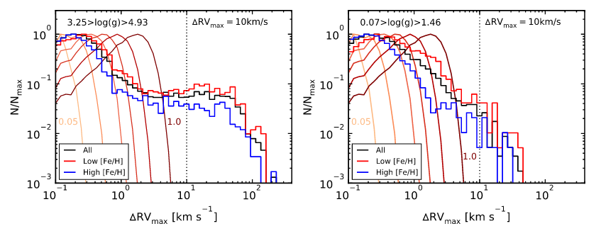
Figure 1: Histogram of the maximal variation in RV between spectra for all stars in the sample. Left panel spans a log g range typical of MS stars, while the left panel includes RGB+RC stars. The black histograms show the whole sample, the red considers only objects with low metallicity (represented by the iron abundance, [Fe/H]), and the blue contains high metallicity objects. The orange plots represent their simulations of what a population of single stars would look like, given the uncertainties in RV, assuming Gaussian errors with σ = 0.05 (lightest shade), 0.1, 0.2, 0.3, 0.5, and 1.0 (darkest shade) km/s. The vertical dashed line represents their conservative limit for a RV variation that can be explained by the uncertainties. Figure 9 in the paper.
It is clear from Fig. 1 that MS stars show higher RV amplitudes than RGB and RC stars. This can be explained by stellar evolution: as stars exhaust H in their cores and leave the MS climbing the RGB, their radii will increase and their log g will decrease. The material will be effectively looser on the surface of the star – in other words, they get closer to overfilling the Roche lobe (limit at which mass transfer begins), which is equivalent to effectively decreasing the orbital distance. As the period is related to the orbital distance, a lower log g causes the period for which binaries remain stable to be lower, thus smaller RV amplitudes are expected.
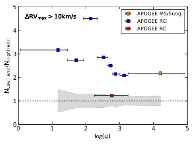
Figure 2: Ratio between the stars with ΔRV > 10 km/s in the low metallicity and in the high metallicity samples, for the different populations. The symbols are placed at the median of each sample, and the horizontal bars give the range of log g values. The shaded gray area is what gives what would be expected from random uncertainties in the measurements. Figure 13 in the paper.
Fig. 1 also seems to suggest that low metallicity objects have higher binary fraction than high metallicity objects. This is a long standing debate, with different studies obtaining different results. Some find that metallicity has no impact on multiplicity, some find low metallicity stars more likely to have a companion, and others found the opposing trend! However, most of this previous studies relied on spectra with lower resolution than APOGEE, which makes it harder to reliably measure both metallicity and RV shifts. To further study the apparent trend in Figure 1, the authors calculated the ratio of stars with ΔRV > 10 km/s between the low and the high metallicity samples, as shown in Figure 2. They obtain that the multiplicity ratio seems to be 2-3 times larger in the low metallicity sample! The exception are the RC stars. However, the existence of the RC itself depends on metallicity: observations show that it is only present in high metallicity populations; low metallicity objects populate the horizontal branch rather than clump. Therefore, it’s easy to explain why the RC does not show the same trend.
The answer to the ultimate question
The effectively estimate the binary fraction, the authors did a simulation and tried to reproduce the observed number of binaries, given the limitations of the APOGEE sampling, with distinct binary fractions. As can be seen in Fig. 3, the multiplicity inferred from observational data is best explained assuming a binary fraction of 0.35. The RC shows a smaller binary fraction, suggesting short period companions were removed during the RGB shell H burning phase (when the star exhausted H in its core, but it’s still burning H in a shell around the He core) that precedes the RC. RGB stars with similar log g to the RC population also seem to break the trend, what is probably due to contamination of RC stars in the sample. Moreover, the higher log g objects seem to show a higher binary fraction. However, this should be interpreted with caution: the APOGEE pipeline was not designed for high log g objects, so the fitted stellar parameters might be subjected to systematic uncertainties.
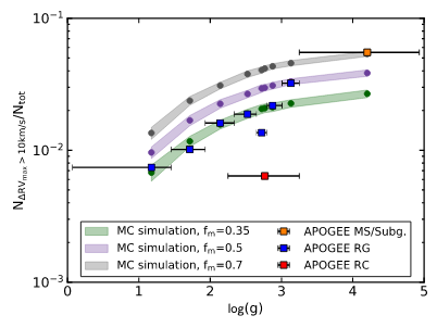
Figure 3: Fraction of stars showing ΔRV > 10 km/s in each log g sample. As in the previous figure, the symbols are placed in the median log g and the horizontal bar gives the range of values. Three simulations done using the Monte Carlo (MC) method with different fractions of multiple systems are shown. Figure 10 in the paper.
With no new observations, but using solely survey data, the authors were able to obtain some enlightening results. As we would expect from theory, observed RV amplitudes depend on the evolutionary phase, with lower log g objects showing smaller amplitudes. They also find that low metallicity objects seem to show a significantly higher binary fraction, what might be telling us something about how the fragmentation of molecular clouds is affected by metallicity. Survey data give the number statistics ideal for this kind of study. Dive in and explore!
Author
Can the log g values be used to derive any sort of mass indicator? Since binarity is apparently strongly correlated with mass, it would be interesting to parse the results in that direction.
Hi there! To get mass out of log g, we would need a radius estimate. We could more or less guess a radius, and even a mass, based on the spectral and luminosity classes (e.g. http://www.isthe.com/chongo/tech/astro/HR-temp-mass-table-byhrclass.html), but then we would be introducing another uncertainty factor, since, as you can check on the linked page, the mass can vary as much as a factor of 5.0 even within a same spectral/luminosity class!
I hope this answers your question!