Title: A Binary Offset Effect in CCD Readout and Its Impact on Astronomical Data
Authors: K. Boone, G. Aldering, Y. Copin, S. Dixon, R. S. Domagalski, E. Gangler, E. Pecontal, S. Perlmutter
First Author’s Institution: Physics Division, Lawrence Berkeley National Laboratory, 1 Cyclotron Road, Berkeley, CA, 94720; Department of Physics, University of California Berkeley, 366 LeConte Hall MC 7300, Berkeley, CA, 94720-7300
Status: Published in Publications of the Astronomical Society of the Pacific [open access]
I’ve lost count of the number of people who assume my job as an astronomer involves peering through a giant telescope all night. This romanticized picture of astronomy is out of date by over a century now, as astronomers were quick to adopt the new technology of photography to make observations repeatable and objective. At first this involved dry plate photography, but since the 1970s virtually all astronomical research has been conducted using charge coupled devices, or CCDs.
CCDs are a remarkable technology, so important that their discoverers won the 2009 Nobel Prize in Physics for the discovery. They do however have some limitations, and astronomers have become very good over the years at correcting for many of the issues they can have. In today’s paper the authors identify a previously-unknown issue with CCDs and set about quantifying its effects in a number of popular instruments and figuring out how to correct for it.
An Analogy: Sprinklers and Buckets
A CCD can be thought of as something like a grid of buckets that each correspond to a pixel in the final image. Imagine someone turning on a garden sprinkler that sprays over the buckets with some fixed pattern. Each bucket will collect different amounts of water depending on the pattern of the sprinkler and its intensity at that point; some will have a lot of water, others little or none. If we then come along and turn off the sprinkler after some time, we could measure the amount of water in each bucket and (in theory) reconstruct the sprinkler pattern.
But instead of measuring each bucket individually, let’s hook up all the buckets in rows. Now we can measure the water in the end bucket of each row, then empty them and move all the water in all the buckets over by one and repeat the process until we’d measured every bucket. As long as we remember which bucket the water we’re currently measuring originally came from (which isn’t too hard) this is a lot simpler than adding measuring devices to every single bucket. How we measure the amount of water in the buckets is also important to understand the issue, and here the analogy breaks down a little, but imagine our water-measuring devices at the end of each row each have a little container holding one gram of water that they use as a reference. To measure a bucket they weigh the water in it against the reference container gram by gram until the amount of water left is less than a gram, at which point they either round up or down and store the number of grams as a binary number (a series of 0’s and 1’s) in a computer somewhere. (In reality, this digitization is forced on us by the quantum nature of the electrons we’re measuring.)
The Issue: Water Where It Shouldn’t Be (and Not Where It Should)
The effect found in the paper is quite subtle. In our analogy, let’s say that we have a sprinkler with a pattern that we know really well, so we can predict exactly how much water should be in each bucket after letting it spray over the grid for a given length of time. We let it spray and subtract the amount of water we know should be in each bucket from all the buckets…then find bits of water left over in some buckets! Some buckets even have less water than they should! (We’ll call this extra or missing water “residual water” because it’s left over after subtraction.) This is similar to what the authors of today’s paper found while working with the SuperNova Integrated Field Spectrograph (SNIFS) on the University of Hawaii 88-inch telescope.
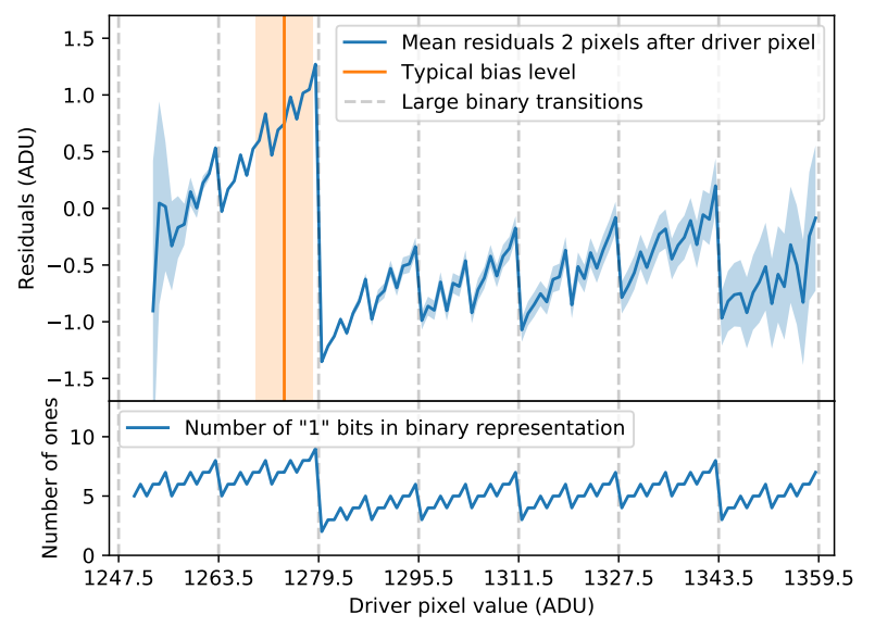
Figure 1: This plot shows the average residual water two buckets after any given driver bucket (top part, blue line), and how the value varies sharply and non-linearly depending on the binary representation of the number of grams of water in the driver bucket (bottom part). Ideally the line in the top part should be flat at zero. Figure 2 in the paper.
Continuing the analogy, they noticed that the residual water in any given bucket seemed to be influenced by the amount of water in the bucket that was measured two spaces before it. (We’ll call the bucket two spaces before the one we’re looking at the “driver bucket,” as it drives the value of later buckets.) They found that the difference in the expected amount of water was proportional to the number of 1’s in the binary representation of the number of grams of water in the driver bucket. Figure 1 shows a clear example of how the changing binary representation of a driver bucket’s value changes the average residual water in a later bucket.
After a lot more analysis the authors concluded that the problem seems to be with the reference grams of water that our measuring devices use. It’s as if while measuring the amount of water in a bucket a few drops of water get added to or removed from the reference gram based on the binary representation of the number of grams of water in the bucket. This then leads to slightly wrong measurements of the next bucket or two; Figure 2 shows this effect clearly. (The analogy really breaks down here, as instead of water it’s electric charge that’s being measured which can effect the reference voltage the measuring electronics use.)
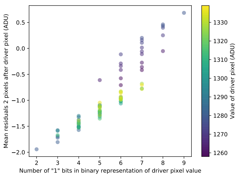
Figure 2: This plot shows the average difference in the number of grams of water (“mean residuals”) found in a bucket two spaces after the driver bucket (“driver pixel”) as a function of the number of 1’s in the binary representation of the number of grams of water in the driver bucket. Note that these are average numbers so they aren’t necessarily integers. Ideally all the values should line up along zero. Figure 3 in the paper.
While the magnitude of the problem may not seem large, it often exists particularly when dealing with boundaries between faint and brighter data, or where the signal-to-noise ratio is low. For instance, it could subtly change the measured shape of galaxies. It’s also pretty widespread; after discovering the problem in SNIFS the authors searched for it in a number of other instruments and found it in several from leading observatories such as the Keck telescopes, the VLT, Gemini, Subaru, and even Hubble. (Though on the bright side they were unable to detect it in a few instruments they checked.)
The Good News: We Can Fix It
Luckily for us the issue is systematic, so once the authors figured it out they were able to develop a process that corrected for the effect in SNIFS quite nicely. They’ve made the code they used to search for its presence in other instruments available on GitHub, so now it’s just up to astronomers to characterize it in other instruments they use and develop corrections for them.
Author
Thanks so much for this extremely well written bite, Daniel! Fascinating
Thanks! I’m glad you enjoyed it. I certainly find in interesting that we’re still learning things about CCDs almost half a century after they were first invented!
The Huntsman Project (https://twitter.com/astrohuntsman?lang=en), building on the Dragonfly Project (http://www.dunlap.utoronto.ca/instrumentation/dragonfly/), should be interested in this given their pursuit of faint low surface brightness data.