Title: A Catalog of Spectra, Albedos, and Colors of Solar System Bodies for Exoplanet Comparison
Authors: Jack H. Madden and Lisa Kaltenegger
First Author’s Institution: Carl Sagan Institute, Cornell University, 311 Space Science Building, Ithaca
Status: Published in Astrobiology, open access
As of today, we have confirmed the existence of 3,774 planets orbiting stars outside our the solar system. Even with the Kepler spacecraft running very low on fuel, new observatories such as TESS (Transiting Exoplanet Survey Satellite) will ensure the number of known exoplanets keeps rising. For many scientists, the next step is not to find more exoplanets but to characterise their physical properties. Are they icy like Enceladus? Or are they rocky like Mars? Do they have an atmosphere capable of supporting life?
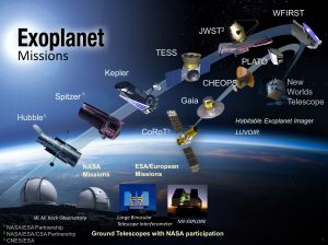
Figure 1: Summary of some past and upcoming exoplanet missions, starting with ground-based observatories like Keck to future missions like CHEOPS. Credit: NASA/JPL-Caltech
The authors of today’s paper have collated the spectra (and albedo) of 19 bodies in our solar system. Using colours alone, they set out to answer an important question – can we distinguish between the three main types of planetary body we see in our solar system: rocky, icy and gaseous?
Colour-colour diagrams
From studying the properties of galaxies to estimating the temperature of a star, colour-colour diagrams are a standard tool in astronomy to compare the apparent magnitude of objects at different wavelengths. There are different methods to do this but in this paper, the authors determine the colour of an object by adding up the flux in its spectrum.
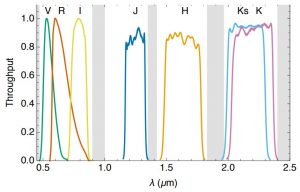
Figure 2: Summary of the filter passbands used to determine the colours of objects. Today we’re focusing on the R-band (orange), J-band (dark blue) and K-band (pink). Figure 5 of paper.A
During this analysis there are two things to keep in mind: 1 – from this data, we cannot distinguish between planet and moon. 2 – as we are only probing their atmospheres, both Titan and Venus are considered to have gaseous surfaces (even though they are both rocky underneath their thick atmospheres). Thus, the bodies are divided in the following manner with moons in italics:
- Rocky bodies Ceres, Io, Moon, Mars, Mercury and Earth
- Icy bodies Dione, Europa, Pluto, Rhea, Callisto, Ganymede and Enceladus
- Gaseous bodies Neptune, Uranus, Titan, Jupiter, Saturn and Venus
Is it Rocky?
Starting with the most familiar body, and maybe the body-type of interest for finding potentially habitable worlds, the authors plot J-K versus R-J for rocky bodies. This is shown below in the right panel of figure 3.
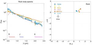
Figure 3: Left we have the spectra for each rocky body, alongside the colour-colour plot on the right. Here, the rocky bodies are grouped in the quadrant where both J-K and R-J are greater than zero. The middle panel of figure 7 from paper.
Here, the rocky bodies are grouped in the quadrant where both J-K and R-J are greater than zero. This is an interesting result for our own planet because its surface is primarily composed of water – not rock!
Is it Icy?
Next up, we have a comparison of J-K and R-J for the icy bodies of our system (note, these are mostly moons) in Figure 4.
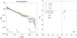
Figure 4: Similar to figure 3, but instead we’re looking at the spectra and colour-colour plot of the icy bodies. This time, the bodies tend to lie in the quadrant where J-K is less than zero, and R-J is greater than zero. Callisto is the odd one out which is sneaking into rocky territory. The bottom panel of figure 7 from paper.
This time, the bodies tend to lie in the quadrant where J-K is less than zero, and R-J is greater than zer0. Callisto is the odd one out and is sneaking into rocky territory, with Ganymede close behind. Both of these moons contain large quantities of dirty snow compared to moons like Europa, thus it makes sense they sit closer to the rocky-icy boundary. It’s anticipated that many exoplanets will also occupy this region.
Is it gaseous?
Finally, we get to investigate the colour-colour magnitude plot of the gaseous bodies – as seen below in figure 5.
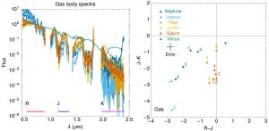
Figure 5: Likewise to figures 3 and 4, we compare the spectra and colour-colour plots of our gaseous bodies. The quadrant of interest is where both J-K and R-J are less than 0 – apart from Venus. Here, Venus is comfortably inside the icy zone. The top panel of figure 7 from paper.
Although most bodies occupy the region where both J-K and R-J are less than zero, several gaseous bodies occupy multiple points on the colour-colour plot. This is because gaseous bodies tend to vary in brightness over timescales shorter than the time between the observations used here – and their spectra change too.
Venus is the odd one out here and is quite comfortably located within the icy zone which is odd considering surface temperatures exceed 700 K. This is because the colour of carbon dioxide atmospheres, like the one surrounding Venus, is very similar to that of an icy surface.
Using colour-colour diagrams, today’s authors have group solar system bodies into three key categories – rocky, icy and gaseous. As exoplanetary spectra become more common and better resolved, this method may prove vital for selecting follow-up targets as we hunt for an Earth 2.0.
Author