Title: Artificial neural network subgrid models of 2-D compressible magnetohydrodynamic turbulence
Authors: Shawn G. Rosofsky, E. A. Huerta
First Author’s Institutions: NCSA, University of Illinois at Urbana-Champaign, Urbana, USA; Department of Physics, University of Illinois at Urbana-Champaign, Urbana, USA
Status: Open access on ArXiv
Turbulence is a fact of life and of physics. You can see it in action when you turn on a faucet, pour cream into your coffee, or simply look up at the clouds. Most of us have an intuitive understanding of what turbulence means: random, chaotic fluid motion that leads to mixing. However, it’s arguably one of the most important unsolved problems of classical physics. A complete description of turbulence is much sought after and accurately simulating turbulence, especially when magnetic fields are involved, is a notoriously difficult problem. Today’s paper explores the use of deep learning techniques to capture the physics of magnetized turbulence in astrophysical simulations.
The onset of turbulence is linked with the Reynolds number of the fluid flow, which is the ratio of inertial forces (associated with the fluid’s momentum) to the fluid viscosity. Viscosity inhibits turbulence. When the Reynolds number is low, viscous forces dominate and the flow is laminar, or smooth. The particles in a laminar flow move more or less in the same direction with the same speed. When the Reynolds number is high, inertial forces dominate and produce eddies, vortices, and other instabilities. This is the turbulent regime, where fluid particles move in different directions with different speeds. The physicist Lewis F. Richardson summarized turbulent behavior with an astute verse:
Big whorls have little whorls
Which feed on their velocity,
And little whorls have lesser whorls
And so on to viscosity.
The image below shows smoke rising from a candle, which starts out as a laminar flow and transitions to turbulent. The Reynolds number can predict where this transition will occur.
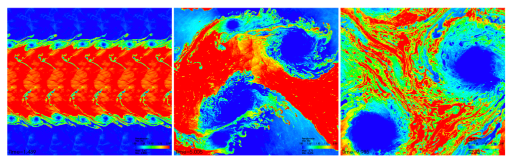
But what does all this have to do with astrophysics, you ask? Most of the baryonic matter in the universe is plasma with a (very) high Reynolds number, meaning that there’s lots of turbulence. So, we need to understand magnetized turbulence in order to understand star formation, solar flares, supernovae, accretion disks, jets, the interstellar medium, and more! The authors of today’s paper are especially interested in magnetized turbulence for the case of binary neutron star mergers. During the merger, turbulence is expected to amplify the initial magnetic field to very high values, which can help launch a gamma-ray burst jet. This happens because of turbulence associated with the Kelvin-Helmholtz instability which develops when two fluids flow past each other with different speeds. Figure 1 shows the development and evolution of the magnetized Kelvin-Helmholtz instability in one of the authors’ simulations.
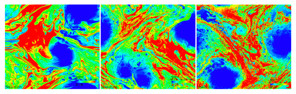
Resolving turbulence and its effects in numerical simulations is a tricky problem. Direct numerical simulations provide the most accurate results but require very high grid resolutions (scaling as the cube of the Reynolds number!) which makes them extremely computationally expensive. In Figure 2, we see three simulations of turbulent mixing that differ only with respect to the grid resolution. The intermediate and high resolution simulations show similar overall behavior but the low resolution simulation looks quite different, indicating that it’s not capturing turbulent effects accurately.
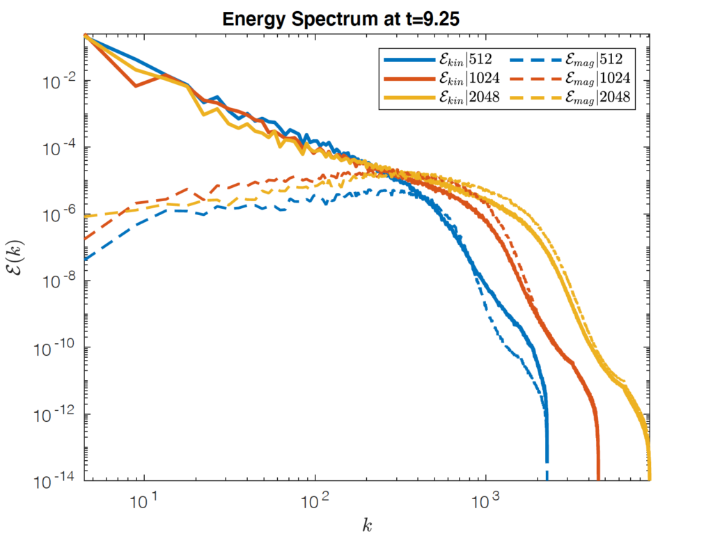
Large eddy simulations are a popular alternative to direct numerical simulations. These resolve only the largest eddies and use a “subgrid-scale” (SGS) model to calculate the contributions from smaller eddies. This greatly reduces computational costs but the accuracy of the simulation depends on the accuracy of the SGS model. The ultimate goal of large-eddy simulations is to reproduce, as closely as possible, the energy spectrum we would obtain in a direct numerical simulation. Turbulence is not simply chaos, and certain statistical properties emerge when we average over time and space. The energy spectrum tells us how energy is distributed as a function of the spatial scale. In Figure 3, we can see the kinetic and magnetic energy spectra for the three simulations shown in Figure 2. Low values of the wave number, k, correspond to large scale features and high values correspond to small scale features. From the figure, we see that the kinetic and magnetic energy spectra do not look the same: the kinetic energy spectrum falls while the magnetic energy spectrum rises as a function of k. This means that small scale (or high k) behavior needs to be modeled carefully to track the overall magnetic energy evolution.
In order for large eddy simulations to reproduce the results of direct numerical simulations, we need to accurately calculate SGS tensors. The objective of today’s paper is to test the suitability of deep learning methods for this purpose. To this end, the authors train a deep neural network to compute the SGS tensor and compare its performance with that of the current state-of-the-art SGS model (the gradient model) which is extensively used in large eddy simulations.
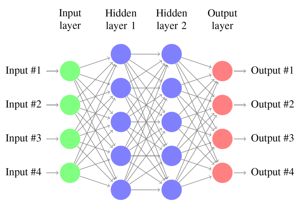
A neural network or net, shown in Figure 4, is a biologically inspired computational model capable of “learning” from data. The basic components of a neural net are called neurons, connected to each other via linear or nonlinear functions resembling synapses. The neurons are arranged in layers and the output of each layer serves as the input to the next. A neural net thus consists of an input layer, some number of hidden layers, and an output layer. A “deep” neural net has two or more hidden layers.
The net creates a relationship between inputs and outputs by adjusting parameters called weights and biases. When the net is training, it is reading in known input-output datasets that constitute the training data, and re-adjusting its parameters to minimize a user-defined cost function. The cost function is a measure of how close the net output is to the correct or desired output. Once the net has been sufficiently trained, it can be used to make predictions for unfamiliar test data. In this paper, the authors used a relatively simple neural network called a multilayer perceptron to implement their model.
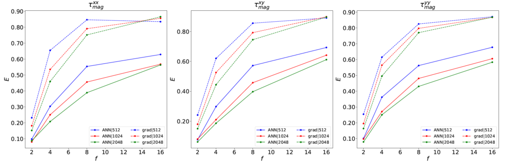
The authors compare the SGS tensors predicted by the gradient model and by a trained neural network with target values calculated from direct numerical simulations. Figure 5 shows the relative error in predicted values for one such tensor. The authors find that the neural network performs significantly better than the gradient model at reproducing SGS tensors, for all tensors and resolutions! This suggests a promising new direction in the development of SGS models for magnetohydrodynamic turbulence.
Given the encouraging results of this a priori study, the authors say the next step would be to implement the SGS neural network model in an actual dynamical simulation and compare it with a high-resolution direct numerical simulation. If neural network models are definitively shown to reproduce the effects of turbulence more accurately than gradient models, it would constitute an important step toward simulating a dizzying array of astrophysical phenomena with higher fidelity. Keep an eye out for more exciting developments on this turbulent front!
Question from one of our students: Does magnetohydrodynamics cover all of the phenomena in plasmas or is it a simpler model for plasmas that doesn’t describe plasma instabilities? This is out of my knowledge range…