Title: Transit Origami: A Method to Coherently Fold Exomoon Transits in Time Series Photometry
Author: David Kipping
First author’s institution: Dept. of Astronomy, Columbia University
Status: Published in Monthly Notices of the Royal Astronomical Society [closed access]
We know that most planets in the Solar System have moons – all except Mercury and Venus – so it seems to follow that exoplanets would have them as well. However, current exoplanet detection methods limit our ability to see these “exomoons”: despite there being over 4,500 confirmed exoplanets, there are only a handful of exomoon candidates, and no confirmations. Astronomers have proposed a few methods to detect exomoons, including potential direct imaging with JWST, and looking for small variations within transit lightcurves. Today’s author explains how one can utilize an altered version of a common method of folding transit lightcurves to find these currently not-so-common signals.
Lightcurves: Folded Up-and-Down or Sideways?
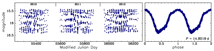
A common method for analyzing exoplanet transit and variable star lightcurves is phase folding. To phase fold a lightcurve, you first estimate a period for the signal through various methods such as periodograms, or by direct calculation (if you have enough information about the system). Then you can divide the time of each data point by the period to get their phase, essentially how far into a periodic cycle the data point is, where a phase of 0.5 represents half a cycle, 1 represents one full cycle, 2 represents two full cycles, etc. Folding the lightcurve allows you to see trends in the data more easily, without really losing any of the other information found within. Figure 1 below shows an example of a lightcurve before and after phase folding, and you can see how the folding transforms it from a jumbled mess to a clear signal.
Instructions for Making an Exomoon
So, how can we use this folding technique to pick out an exomoon signal? According to the author, transit timing variations (TTVs) in the lightcurve – slight differences in the transit center due to gravitational effects on the planetary system, in this case the gravitational effects of the satellite exomoon on the planet – can be utilized to search for exomoons if the main transit signal is first removed. The steps are as follows:
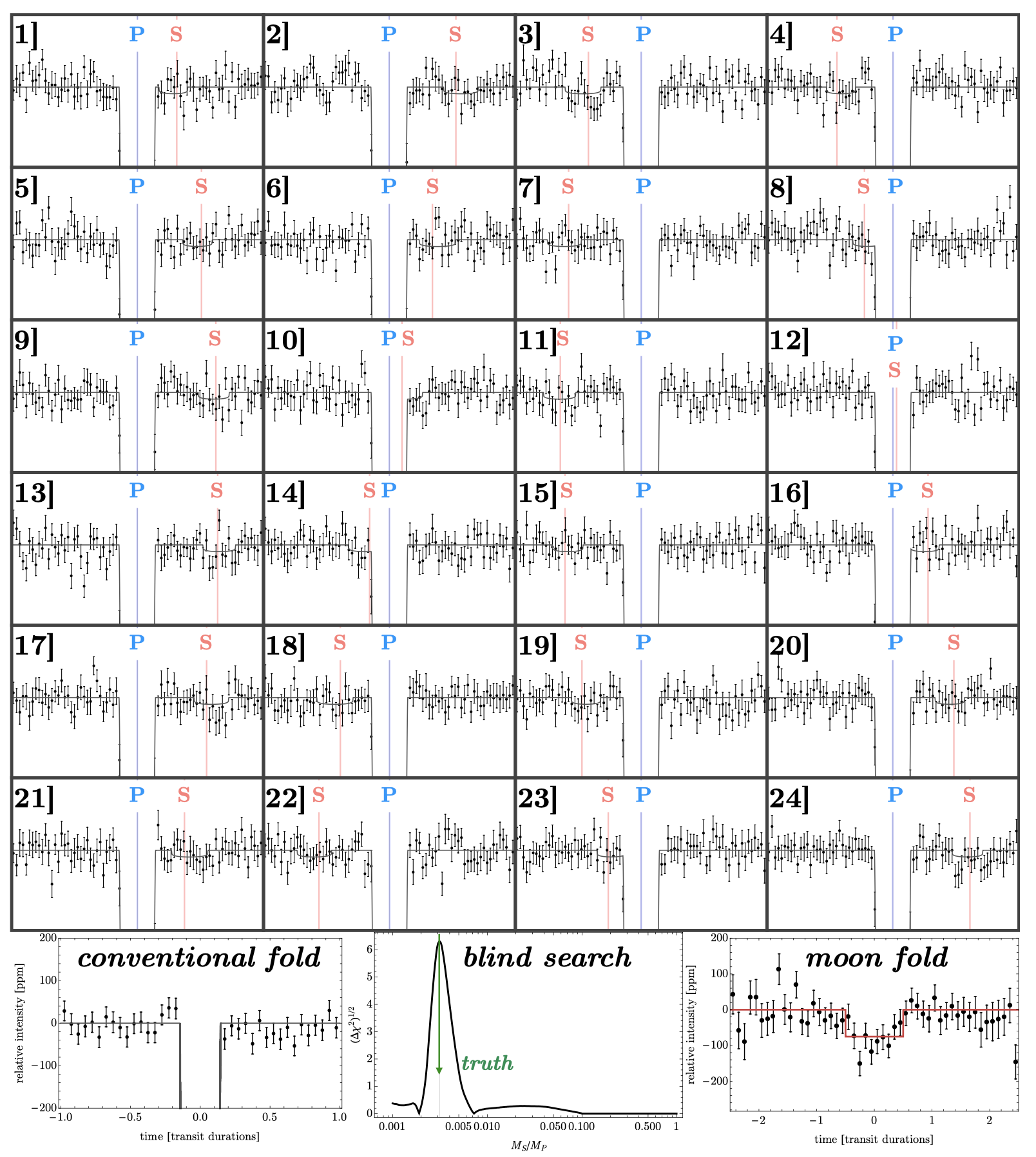
- Determine the time and shape of the transit and lower and upper limits for the first and fourth contact, respectively, then cut everything between those times out of the lightcurve.
- Perform a grid search for the mass ratio between the moon and planet and guess a transit midpoint using a relationship between timing variations, where \(\text{TTV effects on the moon} = -\frac{\text{TTV effects on the planet}} {\text{mass ratio}}\) (Eq. 6 in the paper). Then calculate the moon’s first and fourth contact.
- Find the in-transit and out-of-transit points for the exomoon, combine, calculate a period, and fold.
The author demonstrates his method by a series of 24 synthetic systems (shown in Figure 2) and by analyzing Kepler-973b. In the synthetic systems, he finds that the moon folding method returns the moon signal up to 80% of the time, though the reliability decreases as the inclination of the moon’s orbit increases. In the case of Kepler-973b, he finds that the method could recover an exomoon signal down to an orbital radius of about 15 times the planet’s radius. However, when he works backwards from the mass ratio and estimated planetary radius, he finds that if Kepler-973b’s TTVs were caused by a single moon, it would be too small to be observed. Though it is ultimately a “failed” example, it demonstrates that the method is workable on real data.
There are several caveats to this method. Namely: it assumes that the exomoon will have a similar transit duration to the planet, it requires the exoplanet to have a TTV signal, and it is only effective for exomoons on long orbits around their planets since the signal of the moon can otherwise be blended with the transit. However, if proven effective, the method could help us finally confirm at least a subset of exomoons around giant planets.
Astrobite edited by Ishan Mishra.
Cover Image: NASA, ESA, and L. Hustak (STScI).