Authors: Dang Pham, Lisa Kaltenegger
First Author’s Institution: David A. Dunlap Department of Astronomy & Astrophysics, University of Toronto, 50 St. George Street, Toronto, ON M5S 3H4, Canada
Status: Accepted to MNRAS Letters [closed access]
Water is a key ingredient for life as we know it. In fact, it’s so important that astronomers have a special name for the region around a star where exoplanets can potentially harbor liquid water on their surfaces – the habitable zone. To date, astronomers have found dozens of potentially habitable exoplanets, and hopefully many more to be discovered with upcoming missions such as JWST or HabEx.
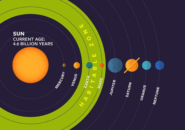
But the key word we need to remember when considering the habitable zone is potentially. If you look at Figure 1 below, you’ll see that in addition to Earth, our moon and Mars are technically within our Sun’s designated habitable zone, though neither are habitable today. In order to understand whether a planet has the potential to harbor life, we need to look further and study its surface and atmospheric composition. This is usually done by analyzing spectra of the planet, which has the downside of being very time-intensive. Given that we have limited time and resources, how should we determine which planets are more likely to harbor water ahead of time, so we can prioritize them as targets for spectroscopy?
The authors of today’s paper test whether it might be possible to look at photometric data from a planet instead – measuring how much flux it emits through different filters – and use machine learning on these fluxes to initially characterize which planets have water.
Shine Bright
The first step in this process is generating a set of ~53,000 cooler, Earth-size planets, which the authors do using a 1D atmospheric modeling software. Next, they dress up their planets with varying fractions of water, snow, clouds, basalt, vegetation, and sand – the major components of Earth’s surface. For each planet, they generate a spectrum of the light it reflects from its host star. Each surface component reflects a different amount of light depending on the light’s wavelength, and we use the term albedo to measure how reflective a certain component is, which is shown in Figure 2. For example, snow is very reflective at shorter wavelengths (signified by a higher albedo), but drops to zero at higher wavelengths, while water’s reflectivity is very low at all wavelengths.
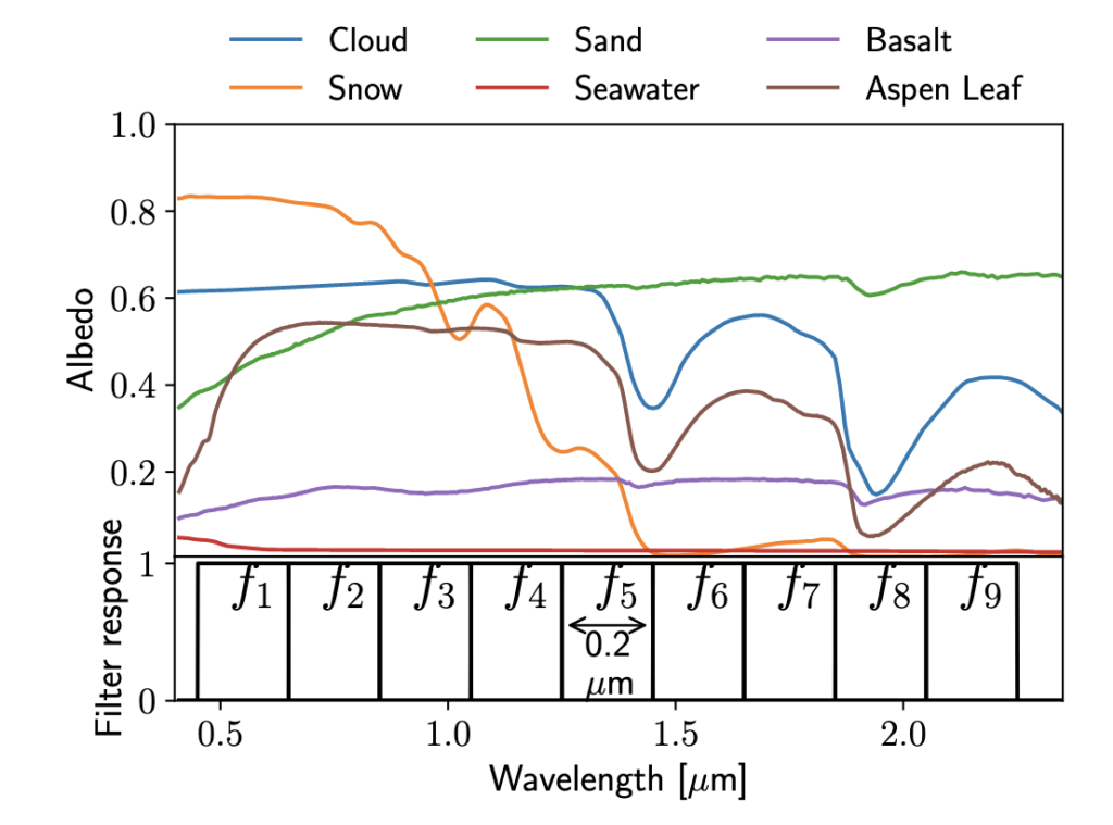
In order to turn these reflection spectra into fluxes, the authors define a set of nine broadband filters, as shown in Figure 2. Each filter is defined such that 100% of the flux from the planet is transmitted (filter response = 1) over a certain range of wavelengths (unlike typical filters where the amount of flux transmitted varies over the wavelength range). They then determine the area under each spectrum with the filters to get the total flux emitted by the planet in each filter, adding in some noise to make it more realistic.
Getting a Boost in Accuracy
Now they are finally ready to put their theory to the test. The authors use a machine learning (ML) algorithm called XGBoost to see if either water, snow, or clouds are present on each planet’s surface. Usually, one can measure how well an ML algorithm works by measuring the accuracy as the fraction of correct predictions out of the total number of predictions made. However, this metric becomes less meaningful if we have an imbalanced dataset. Say we have a bunch of images of apples and oranges that we want our algorithm to identify. If the dataset contains 90% apples and 10% oranges, simply guessing that every image is an apple means that you would measure a highly inflated accuracy of 90%. It sounds like your algorithm is doing great, but in reality it would do no better than a random guess if you had a 50/50 split between apples and oranges. Because this paper’s dataset of water-bearing planets is also unbalanced (a majority of their models have some amount of snow, for example), they instead use a metric called balanced accuracy, which is the (true positive rate + true negative rate) / 2.
We can see their results in Figure 3. Using all nine filters, the algorithm started achieving near perfect BA at a signal to noise (S/N) ratio of ~30 for detecting snow and clouds, and around 0.7 BA for water. The difference in accuracy is due to the albedo effects we saw earlier–water’s reflectivity is very low at all wavelengths and generally appears featureless on a planet’s surface, so it’s much harder to pick out than snow or clouds which have distinguishable features and have a higher albedo.
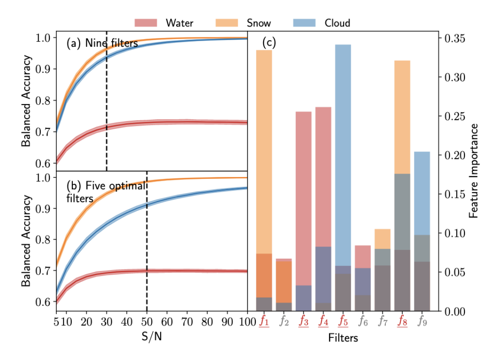
Since most telescopes don’t have nine filters to use, the authors look at their algorithm’s feature importance scores, which are shown in Figure 3c. This tells us which of the nine filters were the greatest influence on the algorithm’s classification, and thus the most important. Using the top five filters with the highest overall importance score, they ran their machine learning algorithm again using only those filters. This is shown in Figure 3b. Though the overall end BA achieved is lower than using nine filters since we’ve lost some data, it still shows a strong performance, achieving asymptotic BA’s around 0.97-1 for snow and clouds and 0.7 for water.
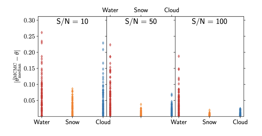
To take it a step further, the authors also run a Markov Chain Monte Carlo (MCMC) simulation using data in the five optimal filters identified before. Instead of just inferring whether or not a water feature is present, the MCMC infers what percentage of the planet’s surface is covered by water, snow, and clouds given the five filter fluxes. They first ran this for just one planet with Earth-like composition and then extended this to 100 random combinations of surface features with varying S/N thresholds. The results from the latter are shown in Figure 4. For each planet and surface element, we see the difference between the percent coverage the MCMC predicted and the actual covered percentage. This residual is once again worse for water, but for a S/N>=50, most predictions were within 5% of true value for snow and clouds and within 20% for water.
All of these results paint a bright picture for using a combination of broadband filter photometry and machine learning for initial characterization of exoplanet surface compositions. This could be a great tool for prioritizing terrestrial exoplanet targets for in-depth, time-intensive spectroscopy, and hopefully in the future large telescopes like LUVOIR or HabEx can run such analyses for the Roman Space Telescope to follow up and open new worlds for us to explore.
Astrobite edited by Lina Kimmig
Featured image credit: Base exoplanet image by NASA/JPL-Caltech/Lizbeth B. De La Torre. Magnifying glass by garnelchen on Pixabay. Composite image with raindrop, snowflake, and cloud done by Katya Gozman.