Title: Pulsar Observations at Low Frequencies: Applications to Pulsar Timing and Solar Wind Models
Authors: P. Kumar, S. M. White, K. Stovall, J. Dowell, G. B. Taylor
First Author’s Institution: Department of Physics and Astronomy, University of New Mexico, 210 Yale Blvd NE, Albuquerque, NM 87106, USA
Status: Accepted to MNRAS
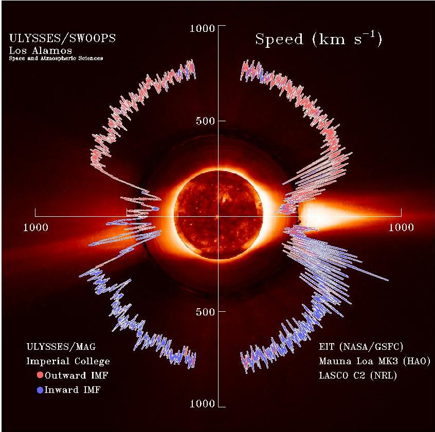
Figure 1: The solar wind is a complicated, dynamic entity, whose properties vary dramatically throughout space. Shown here is a plot of the wind’s speed close to the surface of the Sun, as measured by the Ulysses spacecraft. Image credit: NASA – Marshall Spaceflight Center.
The solar wind is a wild and wonderful thing. It flows through the Solar System, forming graceful cometary tails and beautiful dancing auroras. However, it can occasionally be extraordinarily inconvenient – particularly for radio astronomers, who have to compensate for its subtle effects on their data. Today’s paper discusses the dispersive delay the solar wind imparts on radio signals, possible ways to model and correct it, and the implications for the search for low-frequency gravitational waves.
We sometimes say that the speed of light is a universal constant – and that’s true, but if only we’re talking about the speed of light in a vacuum. If a beam of light is traveling through some medium – air, water, glass, the interstellar medium – it will interact with the particles in the medium, slowing it down. This effect depends on the frequency of the light, so a signal spread across a range of frequencies will appear smeared out, or dispersed, with higher frequencies arriving earlier than lower frequencies.
Since radio waves have very low frequencies, radio astronomers have to deal with dispersion on a regular basis, arising from unbound electrons in the interstellar medium or intergalactic medium. The time delay is typically quantified using something called the dispersion measure (DM), defined as the line integral of the electron number density along the line of sight – in other words, a measure of how much “stuff” is between a radio telescope and the thing it’s looking at. The time delay a photon experiences is proportional to the dispersion measure of the source.
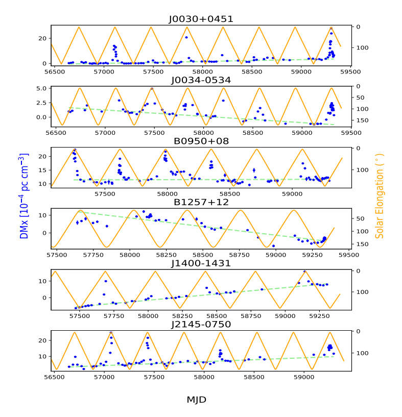
Figure 2: Dispersion measures can exhibit long-term trends, but the solar wind causes additional changes. Seen here are time series plots of the dispersion measures of the six pulsars studied in today’s paper. Each one shows long-term variations in DM, as well as – usually – additional increases when the pulsar appears closer to the Sun. Image credit: Figure 2 from the paper.
It turns out that for broadband radio signals, this delay can be significant, and correcting for it is therefore extremely important. This means that radio astronomers need to know the distribution of free electrons between them and the sources they observe. Over the years, several maps of electrons within the Milky Way have been developed. However, dispersion can arise from any source of free electrons – such as, for example, the solar wind. It, too, needs to be modeled for high-precision observations.
Today’s paper tackles the question of how best to do that. The authors tested out five solar wind models:
- The simplistic model used by the pulsar timing software TEMPO, which assumes the wind to be slow and spherically symmetric.
- The model used by TEMPO’s successor, TEMPO2, which assumes the wind to be fast and spherically symmetric.
- A more complicated spherically symmetric slow-wind model (the “slow” model)
- A more complicated spherically symmetric fast-wind model (the “fast” model)
- The dynamic, numerical WSA-ENLIL model used by the National Oceanic and Atmospheric Administration’s Space Weather Prediction Center, which runs it daily based on up-to-date observations of the Sun.
Testing these models out would require observing radio sources – in this case, rapidly-rotating neutron stars called pulsars – measuring changes in their dispersion measures over a period of time due to the solar wind, and comparing the actual dispersion measure change (“DMx”) to that predicted by the models. Low-frequency data would be best; since a given DMx causes larger time delays at lower frequencies, low-frequency observations are sensitive to small changes in DM. The authors used the Long Wavelength Array in New Mexico to observe six pulsars: five millisecond pulsars (MSPs) and one long-period pulsar, B0950+08. All six lie near the ecliptic, meaning their lines of sight can pass close to the Sun where the solar wind is densest.
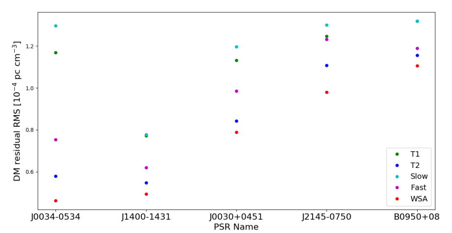
Figure 3: The dispersion measure root mean squared (RMS) residuals quantify how close, on average, a model was to the actual dispersion measures of the sources. The WSA-ENLIL model produced the lowest RMS for every pulsar, meaning that it was the closest to perfectly modeling the solar wind. Image credit: Figure 6 from the paper.
The team found that, for all sources, WSA-ENLIL was more accurate than any of the other models. They also found that default TEMPO model consistently outperformed the “slow” model, and the default TEMPO2 model consistently outperformed the “fast” model. The difference between all five was generally less than a factor of two.
The most interesting implications of this work have to do with pulsar timing arrays (PTAs), ensembles of telescopes which monitor dozens of pulsars and look for minute changes in pulse arrival times caused by nanohertz-frequency gravitational waves. PTAs need to properly model anything that could significantly change the times at which pulses are observed – such, as, for instance, additional time delays caused by DM changes due to the solar wind! The group’s analysis showed that even the four static, spherically symmetry models consistently fell slightly short of reaching the dispersion measure modeling precision PTAs would want to achieve, but that WSA-ENLIL, coupled with low-frequency observations, showed promise. If we want to detect the lowest-frequency gravitational waves in the universe, we need excellent models of the solar wind!
Astrobite edited by Lili Alderson
Featured image credit: NASA – Marshall Spaceflight Center
I’m missing something here – why isn’t the DM measured and corrected for with every Pulsar observation? We do that routinely for dual frequency VLBI and spacecraft range/Doppler observations, and pulsar observation systems tend to have a wide enough bandwidth to determine the DM. The solar plasma delay can change rapidly on short time scales and I can’t believe any a priori model would do that good a job with the plasma delay.
So, you’re right, DMs are measured and corrected for in observations, and those get you DMX time series. The associated uncertainties still end up being a source of noise, though, and fitting to a proper solar wind model reduces that noise (and I’m going to handwave the details away – noise modeling definitely isn’t my specialty, so I intentionally dodged discussing that point). If you want to get into the weeds of how DM variations become noise sources, a paper in the works submitted last fall has a nice section (1.2) that says it better than I could – or at least provides some additional reading on the subject if you have the time.
Thanks for the reference!