Title: The 3D Galactocentric velocities of Kepler stars: marginalizing over missing RVs
Authors: Ruth Angus, Adrian M. Price-Whelan, Joel C. Zinn, Megan Bedell, Yuxi (Lucy) Lu, and Daniel Foreman-Mackey
First Author’s Institution: Department of Astrophysics, American Museum of Natural History
Paper Status: Accepted for publication in AAS Journals [open access on arXiv]
One of the best ways to understand stars is to look at their spectra, which are just plots of intensity of light versus the wavelength. More precisely, we can get a lot from the absorption lines of a star. The absorption lines are caused by cool atoms in the atmosphere of a star that preferentially absorb particular wavelengths, causing that dip in the intensity at that particular wavelength. However, there’s another thing that can affect the wavelength too, and it is called the doppler effect. It is the change in wavelength due to the motion of a star along the line of sight. An object moving towards you has its wavelength shifted to shorter wavelengths, in a phenomenon called blue shift, while an object moving away has its wavelength shifted towards longer wavelengths, which is called red shift. So, this means that wavelengths and the radial velocities of a star are related. Therefore, if we know the wavelength, we can get their radial velocity (we can know how the stars move)! Spectroscopic radial velocities (RV) can be measured and, if available, can already provide a ton of information about stars! There’s a problem: they are not measured for all detected stars, just 7 million of them! Don’t be upset just yet! The researchers from today’s paper were able to infer the velocities of stars that don’t have those measurements. What’s more exciting: if we know the radial velocity measurements, then we can get the ages of the stars (stars are really good at hiding their ages!) using the Age-Velocity dispersion Relations.
To have the 3D vector of the velocities, one needs to measure (or infer in this case) the velocities in x-, y-, and z-directions (in cartesian coordinates). The researchers used the data from Gaia, Kepler, LAMOST and APOGEE catalogs. They used Bayes’ theorem, the way you can infer the posterior probability knowing the prior knowledge of your data. The prior knowledge can be anything from some logical reasoning about the target to the data from different catalogs. The prior helps us to constrain our posterior probability. In the paper, the authors constructed their priors over distance and 3D velocities using the Kepler targets which have RV measurements. They calculated the statistical parameters for stars with measured RVs and then used these parameters to construct a prior over the velocity and distance parameters for stars that don’t have RV measurements.
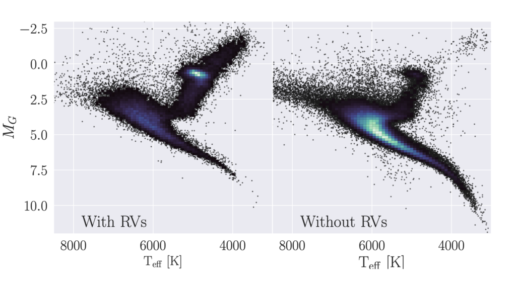
The authors’ goal is to “infer the velocities of stars without RV measurements using a prior calculated from stars with RV measurements.” In Figure 1, you can see the populations of stars with and without RV measurements. The Color Magnitude Diagram helps us classify the stars based on their magnitude and temperature. From that, we know that stars that are higher to the right are upper-main-sequence stars and red giants, and the stars on the tail (as seen on Figure 1) are mid- and lower-main-sequence dwarfs. Therefore, we can see on Figure 1 that stars with RVs (left panel) correspond to giant stars, and the stars without RVs (right panel) correspond to dwarfs. This tells us that there’s a caveat: the stars with and without RV measurements can be from different populations. For this reason, the velocity distributions of stars with RVs will not really help to estimate the velocities of those without.
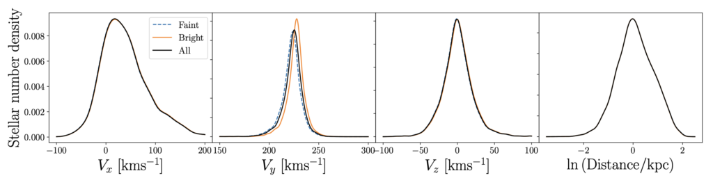
Nonetheless, the velocities in x- and z- directions ended up to be better constrained due to the fact that the y-direction is similar to the radial direction for observers near the Sun and is therefore poorly constrained for Kepler stars without RV measurements. The authors tested this with different choices of priors and confirmed that x- and z- directions of velocities are not really prior-dependent! Meaning, any choice of a prior can constrain the x- and z- directions of velocities. Looking at Figure 2, the first and the third plots show exactly that: the curves are all on top of each other, which shows that the predicted distributions are not dependent on the prior (in this case the priors are the populations of faint stars and bright stars as shown in a figure legend). However, the distribution of inferred y-direction velocities is prior-sensitive. This is because the y-direction is close to the radial direction for Kepler stars as discussed above.
In the end, to validate their method, they compare their inferred velocities with directly-calculated velocities for 5000 Kepler stars with RV measurements. They found that x- and z-direction velocities were inferred more precisely than the y-direction velocities due to, again, the position of a Kepler field (discussed above). Even despite some inaccuracies in y-direction, the inferred velocities are consistent with the true velocities. These inferred velocities therefore can be used to get the kinematic ages of the stars!
Astrobite edited by Lynnie Saade, Briley Lewis, Lili Alderson, Macy Huston
Featured image credit: https://imgflip.com/memegenerator