This guest post was written by Sumit Banerjee, a second year Master’s student at Liverpool John Moores University, UK. Their current research involves studying simulated galactic discs in the ARTEMIS simulations to find signatures of past accretion and merger events. Once obtained, these signatures are then compared with the real evidence of the satellite debris in the real Milky Way Disc. Outside research, they are either working out or speaking at a Toastmasters event.

Title: Employing Deep Learning for Detection of Gravitational Waves from Compact Binary Coalescences
Authors: Chetan Verma, Amit Reza, Dilip Krishnaswamy, Sarah Caudill, Gurudatt Gaur
First Author’s Institution: Institute of Advanced Research, Gandhinagar, Gujarat, India
Status: Submitted
What are gravitational waves and why are they computationally expensive to search for?
“Computers are tired of complex numerical computations. We demand code optimization!!!” claims the furious Computron, head of Global Computer’s Association. I bet if computers were human, this would have been the reality. Computations form the backbone of modern astronomy, and computationally-intensive codes in the field of gravitational wave astronomy come as no surprise.
The science behind gravitational waves (GW) has been around since 1916 when Albert Einstein introduced his general theory of relativity (GR). However, the field of gravitational waves has taken off in the last 5-7 years due to the advancements in technology in experiments like LIGO and Virgo. Gravitational waves were first detected in 2015 and since then, at the time of writing this article, 90+ GW events have been detected by the global network of GW detectors. These GW signals consist of the mergers of binary black holes (BBH), binary neutron stars (BNS) and a neutron star – black hole (NSBH) which could tell us a lot about extreme gravitational fields.
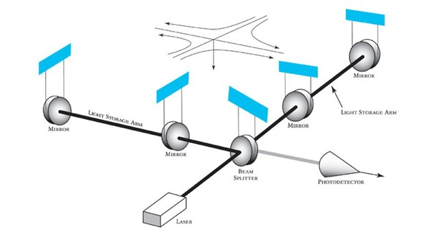
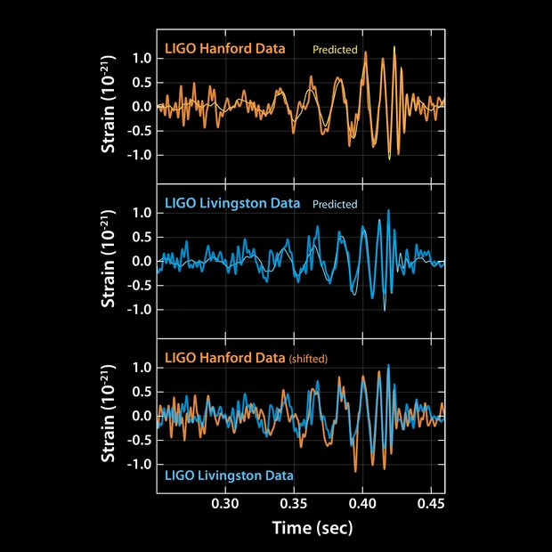
Gravitational waves can be characterized by a quantity called strain, which measures how much the wave stretches and squeezes spacetime. In the detector, this is measured by taking the ratio of how much the length of the interferometer’s arm changes divided by the total length of it. Figure 1 shows the schematic of the interferometer used to detect these waves. The strain could be thought of as the strength of the gravitational wave as a function of time. Figure 2 shows the time varying strain as obtained from the detectors. The strain is then analyzed by the matched filtering technique, the leading computational tool in gravitational waves data analysis. The algorithm correlates the detected signal with a set of template waveforms to see whether the detected strain contains a gravitational wave.
How does matched filtering work?
To understand the algorithm, let us start with an analogy, consider you are visiting your friend for the first time in an unknown city. How would you find your friend? Visit every locality and knock every house to find out where your friend stays. Sounds tedious, right? That’s what matched filtering technique is all about. The idea is to take the strain and compare it with a set of all possible analytical waveforms to see whether the strain has any gravitational wave embedded within it.
Scientifically speaking, astronomers use a bank of analytical wave functions called template waveforms and cross-match the detected signal with every possible template in the bank. Correlating the detected signal with template waveforms is computationally very expensive, leading to latencies in computing gravitational waves. The obvious question – could this be improved? In principle, yes. To understand how, let’s get back to your friend’s search. Imagine that now you know the locality, say “Park Street ” and the house number (HU-207). Finding your friend becomes easier and takes less time because the search area has reduced. Can we do something similar with matched filtering? The answer is yes, and it has to do with deep learning.
How do we make the computations less expensive?
A team of astronomers at Institute of Advanced Research in India have explored this idea and have developed an algorithm that serves as a balance between computation and existing deep learning models to reduce the number of computations needed to analyze the detector signal.
Stand-alone deep learning models treat analysis of gravitational waves as a classification problem. On one hand, this is less computationally-expensive, but it does depend on the availability of training data; if the models aren’t trained on enough data, they might misclassify noise as a gravitational wave signal or vice versa.
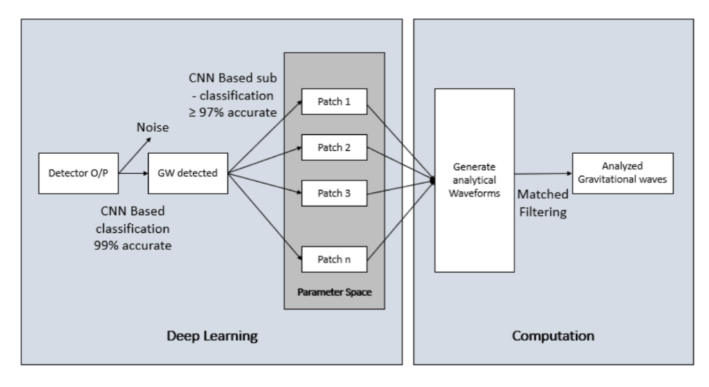
The paper covered in this article describes a method of using both deep learning models and computations to study gravitational waves. They perform this in several steps:
- Step 1: A trained convolutional neural network is used to check whether the detector output has a gravitational wave signal. This step separates noise and GW signals, if present.
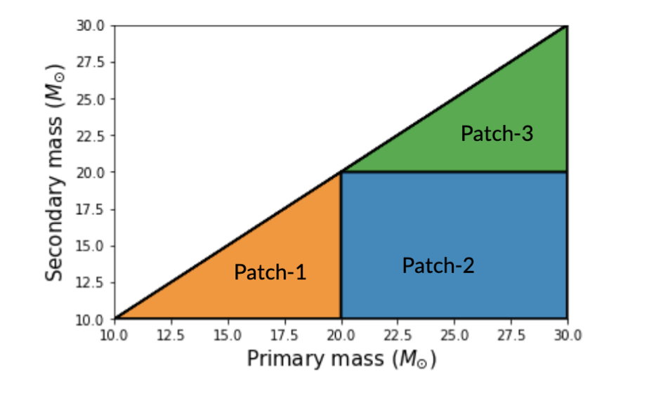
- Step 2: The parameter space (which consists of all possible parameters along with their allowed values) is divided into patches to narrow down the possible combinations. This is similar to getting a locality and a house number while searching for your friend in the unknown city. Figure 3 shows an example of how patches in the parameter space are obtained.
- Step 3: With the gravitational wave detected in Step 1 and the patches obtained in Step 2, the trained neural network then finds out to which patch the signal belongs to. Let us assume that the network classifies the signal as being in Patch 1.
- Step 4: Analytical waveforms are generated against every template point in Patch 1. Given that our example signal from Step 3 is in patch 1, the analytical waveform corresponding to a primary mass of 15 solar masses and secondary mass of 12.5 solar masses is a valid waveform whereas an analytical waveform corresponding to a primary mass of 25 solar masses and secondary mass of 15 solar masses is not given that the signal is in Patch 1.
- Step 5: The cross-matched filtering is performed on the set of waveforms generated in Step 4 above. Since a reduced area of the parameter space is searched, there is a significant reduction in the number of computations required, thus improving latency.
Did deep learning help?
To test the effectiveness of this hybrid approach, synthetic signals were generated and the system was allowed to study them. The model separated out noise from noisy BBH signals with an accuracy of 99% and obtained an average accuracy of ≥ 97% when classifying the detected signals in one of the patches in Figure 3. That is, if a signal belonged to patch one for instance, the algorithm classified the signal as belonging to patch one 97% of the time. The initial results look promising and the authors have expressed their willingness to develop the method further with the ultimate goal of designing low latency algorithms for GW signal identification.
In summary, computations are expensive and deep learning models are not reliable. As per the current situation, the analysis of signals containing a gravitational wave still relies on computations, but the algorithms in this paper provide a quicker way of analyzing them, which could bring in code optimization as demanded by the furious Computron.
Astrobite edited by: Haley Wahl
Featured image credit: Sumit Banerjee