Authors: CHIME Collaboration: Mandana Amiri, Kevin Bandura, Arnab Chakraborty, Matt Dobbs, Mateus Fandino, Simon Foreman, Hyoyin Gan, Mark Halpern, Alex S. Hill, Gary Hinshaw, Carolin Höfer, T.L. Landecker, Zack Li, Joshua MacEachern, Kiyoshi Masui, Juan Mena-Parra, Nikola Milutinovic, Arash Mirhosseini, Laura Newburgh, Anna Ordog, Sourabh Paul, Ue-Li Pen, Tristan Pinsonneault-Marotte, Alex Reda, J. Richard Shaw, Seth R. Siegel, Keith Vanderlinde, Haochen Wang, D. V. Wiebe, Dallas Wulf
First Author’s Institution: Department of Physics and Astronomy, University of British Columbia, Canada
Status: Published in ApJ [open access]
A Map of the Universe
Throughout the history of astronomy, we’ve been able to map the universe in a couple of different ways. Large surveys of galaxies, such as SDSS or DESI are extremely useful – they give astronomers a huge sample of galaxies to characterize, and the positions of those galaxies tell us things about how the universe as a whole is set up. At extremely high redshifts, the Cosmic Microwave Background (CMB) shows us the structure of the universe right as it began. More recently, a totally separate technique has been developing: (spectral) Line Intensity Mapping (LIM). In this technique, you essentially take a very blurry picture of a large region of the universe, at wavelengths that correspond to a specific spectral line. Instead of targeting specific galaxies, you get all of the emission from that spectral line in that region of the universe. This way, you can get light from things that are much fainter than a traditional galaxy survey can see.
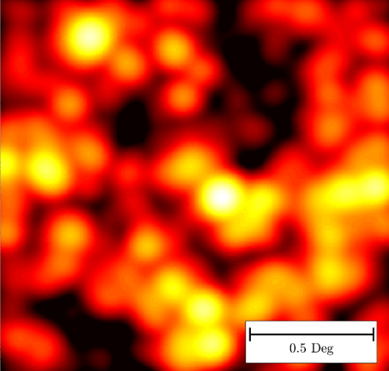
The fact that you’re targeting a specific spectral line is also important: because of the expansion of the universe, emission from different distances is redshifted to different observed wavelengths, and so the end product of a LIM experiment is a 3D map of the universe, instead of just a 2D picture. Because of the expansion of the universe, this also means you map the universe through time. Figure 1 shows a (very idealized) picture of what a single wavelength slice of this could look like.
Neutral About Hydrogen
The LIM technique was originally developed for studies of the 21 cm Hydrogen line, which is a spin-flip transition of neutral hydrogen (HI) and is mainly emitted by diffuse gas. This is a very powerful technique: it’s extremely difficult to observe neutral hydrogen gas in any other way, and a lot of the universe is made up of this gas, especially at high redshifts!
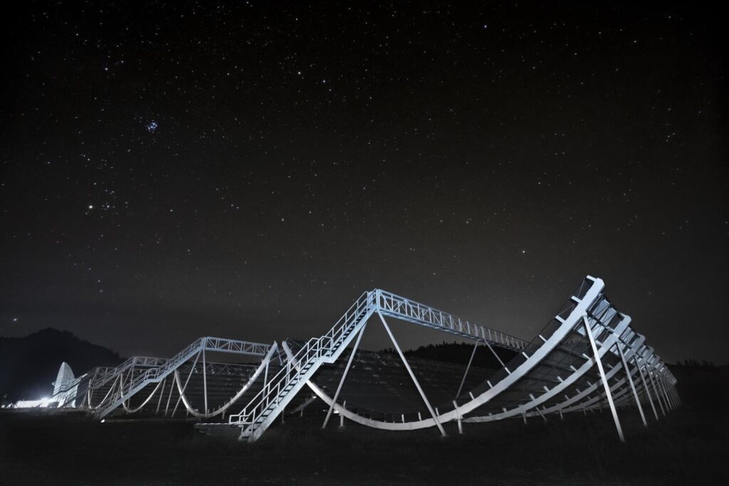
Today’s paper is also looking for this 21 cm emission, specifically by using the Canadian Hydrogen Intensity-Mapping Experiment (CHIME; shown in Figure 2). This experiment has been discussed in several astrobites over the past few years, both for its 21 cm work (x) and for its work with Fast Radio Bursts (x, x, x).
Fighting Foregrounds with Friends
Detecting 21 cm is significantly complicated by the fact that there are lots of things in the way! Between Earth and the distant galaxies astronomers are actually after, there are many other sources that emit around 21 cm wavelengths, including the Earth’s ionosphere and synchrotron emission from the Milky Way. These are ‘foregrounds’, and they’re far brighter than the 21 cm emission astronomers are looking for! Although you can work around foregrounds using 21 cm data alone, combining your 21 cm measurement with other measurements of the structure you’re trying to see (taken using other wavelengths of light) makes for a much more robust approach. Because the two measurements are taken using different wavelengths, it’s very unlikely that they’ll show the same foreground structure. When you use a statistical technique such as cross-correlation to combine the two, the foregrounds (more-or-less) disappear! This has already been done for the CHIME 21-cm data at low redshifts, but not at redshifts above 1.5 (9 billion years ago).
In this paper, the authors combine their 21 cm data with Lyα forest measurements from eBOSS (the extended Baryonic Oscillation Spectroscopic Survey), which is a part of SDSS. Importantly, the Lyα forest traces absorbing hydrogen gas, and the 21 cm data traces emitting hydrogen gas. Density determines whether gas absorbs or emits: denser gas tends to absorb radiation, and more diffuse gas tends to emit radiation. This means that on small scales, the two signals are actually expected to be anti-correlated (because the measurements are coming from different kinds of gas), and the cross-correlation signal will be negative.
A Negative Detection!
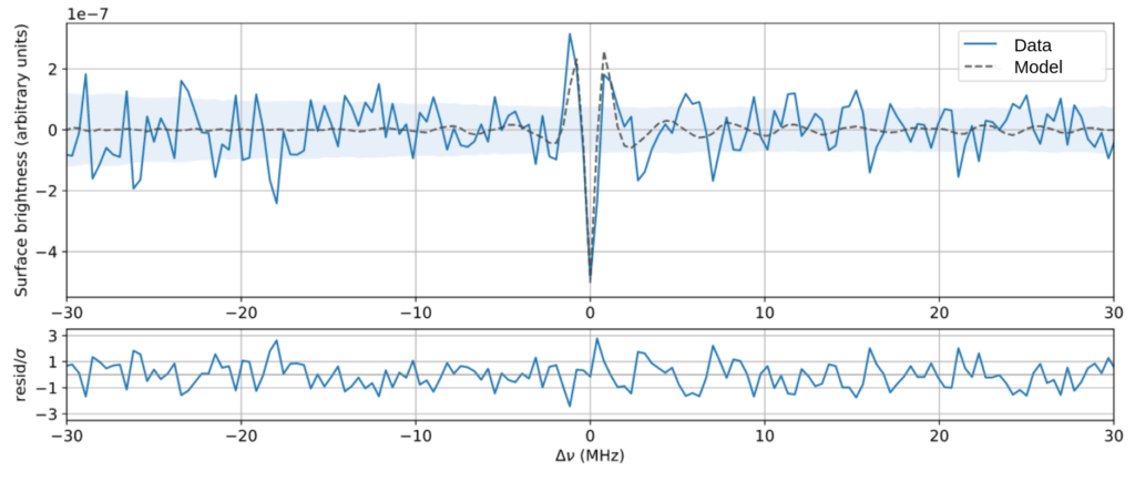
Indeed, after reducing the CHIME 21 cm data, the authors do detect anticorrelation! Figure 3 shows the cross-correlation signal. This is measured by introducing an artificial offset between the 21 cm measurement and the Lyα forest measurement in the x-axis (in this case, the frequency axis), and then measuring how much they correlate or anti-correlate at that offset. The amount of correlation is then shown as a function of this frequency offset. You can see a large negative spike right at zero offset, where the two signals should anti-correlate the most. The dotted black line shows a model the authors came up with for this cross-correlation, and the two agree quite well (the bottom panel shows the residuals between the signal and the model).
This is very exciting – it’s the first detection of 21 cm signal at redshifts greater than 1.5, and its cross-correlation with the Lyα forest looks pretty much as expected! There is a lot of information to be gained from this measurement. In particular, the amplitude in the y-axis of the cross-correlation signal is set by the spatial relationship between dense and diffuse hydrogen gas in the universe. However, the authors leave determining that exact relationship for a future work, because it requires some extremely detailed cosmological and hydrodynamical simulations. Also, even in this cross-correlation measurement, the authors found a lot of foreground emission! Improvements to the CHIME instrument and its data reduction will help get rid of this contamination in the measurement, but it’s still a very difficult problem. For now, it’s incredible that this faint but all-important signal has been detected, so far away.
Astrobite edited by Nathalie Korhonen Cuestas
Featured image credit: Volker Springel (Max Planck Institute for Astrophysics) et al.