Mathematics is often accused of being too esoteric and abstract to matter in everyday life – even by astronomers – and maybe this is a valid criticism. In the real world, a neighborhood is where your house is; the Riemann zeta function is the sorority formal you attended last week; and a Lie group is a pyramid scheme your ex-high school classmate is asking you to join. However, the branch of differential equations stands apart, as we can’t get through a single day in our ever-changing universe without seeing their effects. Anything and everything undergoing any sort of change, from the temperature of your lap as your cat naps in it to the size of the universe, is governed by differential equations. Differential equations come in two main flavors: ordinary differential equations (ODEs), your bread-and-butter single variable situation (like dropping an egg off the roof), and partial differential equations (PDEs), the multi-variate scenarios (like dropping an egg attached to a magnet off the roof, directly into an electromagnetic field), which quickly become too messy for neat analytic solutions. Here, we present a definitive ranking of the top ten differential equations in astronomy and astrophysics!

#10: The Klein Gordon Equation

\((\text{☐}+m^2)\psi = 0 \)

Quantum mechanics (QM) — the theory that explains the probabilistic behavior of particles — and special relativity (SR) — the theory that corrects Newtonian physics for objects in non-inertial reference frames — are natural enemies. One of the fundamental tenets in SR is that we live in four dimensional space-time, where time stands on equal footing with the three spatial dimensions. However, the Schrödinger equation (the differential equation describing the behavior of a particle) treats time and space very differently! However, the disconnect between QM and SR should be fine as long as our particles stay well below the speed of light…but wait — light itself is a particle. Schrödinger himself tried to fix this by squaring his QM equation (shortened with the trendy ☐ operator), which gave us the Klein-Gordon equation. However, he decided it was too good to be true, and gave up. Decades later, the Klein-Gordon idea came back to life in relativistic quantum theory, and we include it on this list as a reminder to all despondent astronomy students thinking about giving up on their research ideas.

#9: The Lane-Emden Equation

\(\frac{1}{\xi^2}\frac{d}{d\xi}\left(\xi^2\frac{d\theta}{d\xi}\right)+\theta^n=0 \)

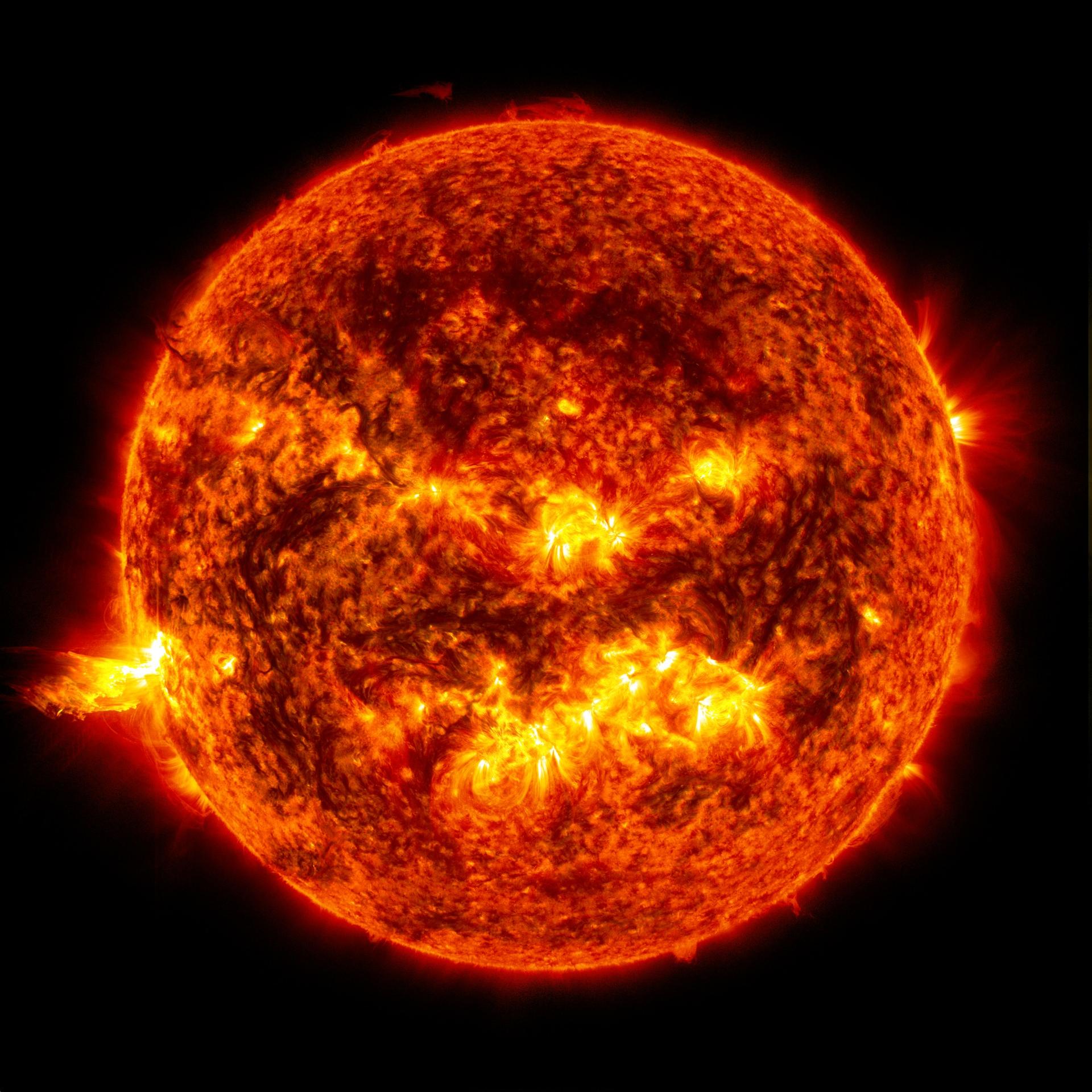
Have you ever wondered how the density of a star changes as you move inward from its surface? If so, well — the Lane-Emden equation has your answer! If not, then the Lane-Emden equation is here to remind us that stars can be interesting! The little exponent \(n\), known as the polytropic index, depends on the relationship between pressure and density inside the star. It may look harmless, but don’t be fooled — \(n\) is packed with physical meaning. If our star has a constant density throughout (unrealistic unless you’re modeling a rocky planet instead), \(n=0\). If we have a neutron star, \(n=1\), and if we have a star with an infinite radius (though I certainly hope not), \(n=5\). In these cases, the Lane-Emden equation can be solved. If you’d like to model any other star, such as our Sun, you can integrate all you’d like, but you won’t find an analytical solution.

#8: Three (Similar Size) Body Equation of Motion

\(m_1\frac{d^2\mathbf{x}_1}{dt^2}+m_1m_2G\frac{(\mathbf{x}_1-{\mathbf{x}}_2)}{|{\mathbf{x}}_1-{\mathbf{x}}_2|^3}+m_1m_3G\frac{({\mathbf{x}}_1-{\mathbf{x}}_3)}{|{\mathbf{x}}_1-{\mathbf{x}}_3|^3}=0\)

Celestial mechanics is perhaps the simplest subfield of astronomy – there is (almost) always only one force at play, and it’s one we all know quite well: gravity. The equation of motion (EoM) that governs two objects orbiting each other (such as the Sun and Jupiter) will always have a tidy solution; if we throw in a third, much less massive object (such as Earth in the Sun-Jupiter system), the EoM will still yield a well-behaved, predictable solution (albeit with some quirks, such as the Jupiter-induced gaps in the asteroid belt and the stable solar orbit a million miles away which is now home to JWST). However, if this third object is not much less massive (such as if we added an additional star to our Solar System), the results are much more exciting. This equation has no analytical solution, and the behavior of the system is entirely chaotic and unpredictable! We are lucky our Sun is a loner (unlike most stars, which have at least one companion), otherwise our clean, nearly circular orbit wouldn’t exist!

#7: The Navier-Stokes Equation

\(\frac{\partial \mathbf{u}}{\partial t}+(\nabla \cdot \mathbf{u})\mathbf{u} = -\frac{\nabla P}{\rho}+\frac{\nabla \cdot \mathbf{\tau}}{\rho}+\mathbf{a} \)

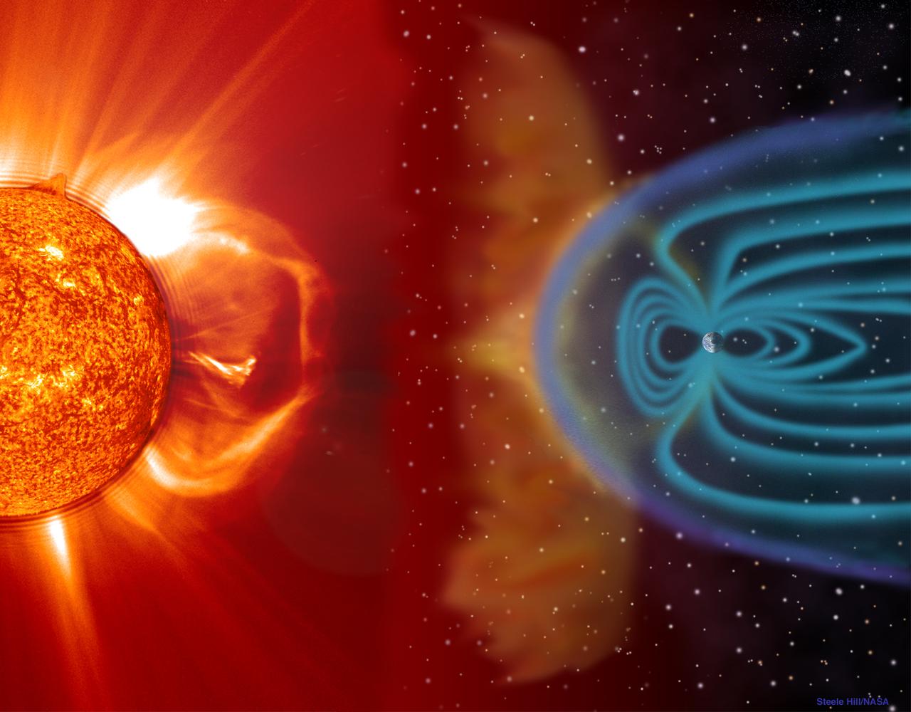
The holy grail of astronomers modeling planetary atmospheres and supermassive black hole accretion disks alike, the Navier-Stokes equation describes the behavior of and plasma. If your theorist friend is hogging all the CPUs on the computing cluster, it is very likely they are attempting to numerically solve this equation. Fluid mechanics is inherently tricky; not only do the properties of a fluid change throughout its volume and over time, but any tiny parcel of fluid is constantly moving. It never sits still. On top of that, we have to worry about pressure, stress, and other force changes throughout the fluid! The solutions get especially messy if the fluid is turbulent (it flows unpredictably); while your first instinct may to want nothing to do with the Navier-Stokes equation for a turbulent fluid, the Solar System as we know and love it could not have formed without turbulent gas and dust!

#6: The Euler-Lagrange Equations

\(\frac{\partial \mathcal{L}}{\partial q}=\frac{d}{dt}\left(\frac{\partial \mathcal{L}}{\partial \dot{q}}\right) \)

Are you tired of dealing with confusing coordinate systems, accounting for annoying vectors, and figuring out all the forces acting on your system? If so, you need look no further than the Euler Lagrange equations! This way, you can easily derive the equation of motion for your system in minutes, and even give a relativistic particle the quantum mechanical treatment! All you need is the difference between the kinetic and potential energies in your system (known as the ever elegant Lagrangian) in terms of your choice of generalized position (denoted \(q\)) and velocity (denoted \(\dot{q}\)). Not only are the Euler-Lagrange equations a clever alternative to your traditional Newton’s second law, but as mathematical physics girlboss Emmy Noether proved, for every \(q\) or \(\dot{q}\) not appearing in the Lagrangian, there is a corresponding quantity in your system which is conserved!

#5: Maxwell’s Equations

\(\nabla^2\phi-\frac{1}{c^2}\frac{\partial^2\phi}{\partial t^2}=-4\pi\rho \)

\(\nabla^2\mathbf{A}-\frac{1}{c^2}\frac{\partial^2\mathbf{A}}{\partial t^2}=-4\pi\mathbf{J} \)

Maxwell’s equations are the Newton’s laws of electromagnetic fields, which are essential in astronomy, whether we’re counting photons with our telescopes or tracing the origin of incoming cosmic rays. Traditionally, there are four, and they are written in terms of the familiar electric and magnetic fields, \(\mathbf{E}\) and \(\mathbf{B}\), respectively. However, these would definitely not make this list, especially not with the dreadfully boring \(\nabla \cdot \mathbf{B}=0\) showing up just to ruin magnetic monopoles for everyone. If you abstract them into the field potentials, \(\phi\) and \(\mathbf{A}\), so you don’t get distracted by trying to reconcile your differential equations with something mundane and important to every day life, like electricity, Maxwell’s equations become much more satisfying.

#4: The Free Particle

\(\nabla^2\psi(r,\theta,\phi)=E\psi(r,\theta,\phi) \)

The free particle — completely unrestrained by external forces — is truly an enigma. In classical mechanics, its behavior is completely trivial: according to Newton’s first law, it will travel forever in a fixed direction at a fixed speed. However, when approached from a quantum mechanical perspective, the free particle is wildly problematic. It will go wherever it wants, challenging the idea that the probability of finding it somewhere in space should add up to 100%. Better yet, the solutions to the quantum free particle equation are spherical Bessel functions, perhaps the most esteemed of the special functions, which are exact functions, despite lacking a closed form.

#3: The Radiative Transfer Equation

\(\frac{dI_\nu}{ds}=-(\alpha_\nu+\sigma_\nu)(I_\nu-S_\nu) \)

As astronomers, we are almost always trying to determine the brightness of some astrophysical phenomena. Unfortunately, three pesky behaviors of light are constantly getting in the way: emission, when light is created; absorption, when light is destroyed; and scattering (a whole can of worms on its own), which leads to pinging photons around and changing their energies. The radiative transfer equation is then our best friend, enabling us to untangle the possible modifications of our brightness measurements.

#2: Bremmstrahlung-Produced Photons

\(\frac{d^2n_\gamma}{dtdk}=\int{n_e(E)\frac{d^2n_i}{dtdk}}dE \)

Sometimes, we may find ourselves in a situation with lots of high energy electrons, and we want to know what, exactly, is going on. This is tricky, since these particles can be quite social (and violent!), and can collide with one another or get spun around by strong magnetic fields, and all we have to study them is the light (and occasionally, neutrinos!) they emit. In this case, it is helpful to determine the expected number of emitted photons at a given time and frequency, which is observable here on Earth, given a model of the distribution of electrons and a dominant electron interaction mechanism. Unfortunately, the solution is never straightforward, regardless of your choice of model parameters. However, in a system where most electrons lose a substantial amount of their energy in every interaction (such as through the notorious Bremsstrahlung radiation, whereby a nearby ion snatches the energy away), the relation isn’t even a differential equation! It is an integro-differential equation, which some may say is unnatural, or dangerous, like mixing bleach and ammonia. However, real calculus enthusiasts would say it combines the best of both worlds (integration and derivation) in a problem sure to keep you busy all day.

#1: The Hydrogen Atom

\(\nabla^2 \psi(r,\theta,\phi)+\frac{\psi(r,\theta,\phi)}{r}=E\psi(r,\theta,\phi) \)

The equation describing the behavior of an electron in the hydrogen atom is an all around top-tier differential equation – and that’s why it earns the #1 spot on this list. For one, hydrogen is the only element for which the Schrödinger equation has an analytical solution. It also happens to be the most abundant element in the universe, making this equation foundational for understanding everything from stars to interstellar clouds. What really sets it apart, however, is that it is a true triple threat: a partial differential equation with three variables, the solution is a product of special functions, the spherical harmonics and the Laguerre functions!

Honorable Mention

To balance out the likely criticism that this list is biased toward special functions, we close with a shortlist of fan favorites from the Penn State Astronomy Department. The wave equation is a recurring favorite: department head Randy McEntaffer says the human interpretation of photons is very intriguing, and graduate students Lukas Stone and Kadri Nizam bonded over writing a code to find its solutions numerically. Professor Mike Eracleous supports the Bessel differential equation, not for its application to the free particle, but for diffraction of light. Lastly, from the practical professors: Caryl Gronwall argues the Newtonian equation of motion for gravity deserves the top spot, since it affects us every day here on Earth, and Robin Ciardullo prefers any differential equation which is easy and solvable (a narrow list!).

Edited by Niloofar Sharei