Authors: Stanway, E. R., Byrne, C. M., & Upadhyaya, A.
First Author’s Institution: Department of Physics, University of Warwick, Gibbet Hill Road, Coventry CV4 7AL, UK
Status: accepted to MNRAS [open access]
The Birth of Stars
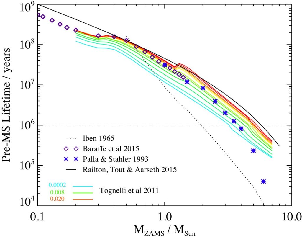
Stars form from clouds of molecular hydrogen that collapse under the force of their own gravity. As the gas collapses, it heats up until the temperature and pressure at the core of the cloud is high enough for hydrogen to fuse into helium. The onset of hydrogen fusion marks the moment a star is born, and from that moment, until the time that the star runs out of hydrogen, the star is said to be on the main sequence. More massive clumps of gas have a stronger gravitational force, and therefore collapse much faster than less massive clumps of gas. For example, it takes a cloud of gas less than 1 million years to collapse into a star more than five times as massive as the Sun, whereas it takes over 100 million years to form stars less than half of the mass of the Sun.
Scaling up to millions and billions of stars
Using our understanding of star formation and stellar atmospheres, astronomers can model the light emitted by a simple stellar population (SSP), or a group of stars which were all formed at the same time. Models of stellar evolution can also be used to predict how this SSP will change over time as stars evolve off of the main sequence, begin fusing heavier elements, and eventually die. Combining different SSPs then allows astronomers to model more complex and realistic stellar populations. This technique, known as stellar population synthesis, is a cornerstone of modern astronomy, and can be used to predict the rates of supernovae explosions in the universe, measure the mass of distant galaxies, and reconstruct the star-forming history of a galaxy.
In building an SSP, an astronomer must make many different choices, all of which will have a systematic effect on the resulting predictions. Which library of evolutionary models should you use? How many stars are in binaries? What is the distribution of stellar masses? It’s impossible to account for every single variable affecting star formation, so some simplifying assumptions have to be made.
Forming stars in an instant!
One assumption that is often made in SSP modelling is that all stars, regardless of their mass, are formed at the same time. However, we know that this is not the case, since low-mass stars take a lot longer to form as compared to high-mass stars.
Today’s authors examine how the results of stellar population modelling may be affected by accounting for the delayed formation of low mass stars. For the first time, they combine models of stars’ pre-main-sequence (pre-MS) lifetimes (Figure 1) with Binary Population and Spectral Synthesis (BPASS) stellar evolution models and spectra. They followed the evolution of a single stellar population over 20 billion years to investigate how the number of stars of different masses and the light they output is affected by the pre-MS delay of low-mass star formation, and also applied these models to a mock galaxy observation.
Effects On A Single Stellar Population
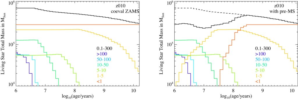
Today’s authors consider two stellar populations, which form the same total number of high and low-mass stars over time. In the first population, all stars are formed at exactly the same time, but in the second population, they incorporate a realistic pre-MS delay so that low-mass stars are formed after high-mass stars.
Incorporating a pre-MS delay has a significant effect on the distribution of masses present in a stellar population. In the case of where all stars are formed at exactly the same time, low-mass stars contribute much more to the stellar mass than high-mass stars do, from the very beginning. This is because many more low-mass stars are formed as compared to high-mass stars. You can see this in the left panel of Figure 2: the orange and red curves (low and intermediate mass stars) are far above the blue curves (high mass stars) at every age (x-axis). High-mass stars burn through their fuel very quickly and die in high-energy supernova explosions not long after they are born. This is why the blue curves very quickly drop towards 0 in both panels of Figure 2. Lower mass stars, on the other hand, have much longer lifetimes, and hence their contribution to the total stellar mass remains about constant.
Once the authors incorporated a pre-MS delay to star formation, the relative contributions of low and high-mass stars to the total stellar mass changed subtly. Although the total number of low mass stars formed is still much higher than the total number of high mass stars, many fewer low-mass stars are born before high mass stars die in supernovae. As a result, the stellar population is more strongly dominated by high-mass stars at early times when accounting for the delay to low-mass star formation.
The mass of a star strongly affects its spectrum, or, how much light it emits at each wavelength. A high-mass star emits much more light, especially at short, energetic ultraviolet wavelengths, than a lower-mass star, which emits more of its light at longer, less energetic wavelengths in the optical and near-infrared. The pre-MS delay means that lower-mass stars start producing optical and infrared light at later times, making the total amount of optical and near infrared light produced by a stellar population 10-15% lower at early times (less than 1 million years after the beginning of star formation).
Galaxy-Scale Effects
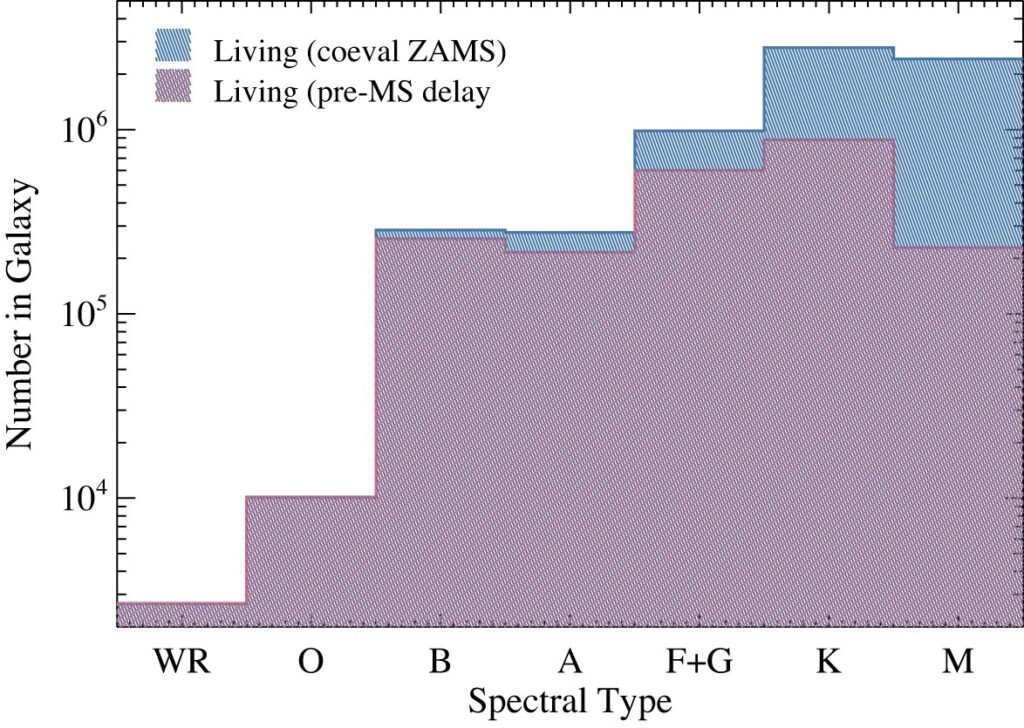
To put their results into context, the authors explored the effects of a pre-MS delay on a simulated galaxy. They chose a galaxy produced by the Feedback In Realistic Environments (FIRE) simulation, which has formed about 12.5 million solar masses worth of stars over ~316 million years. The authors then modelled the stellar population of the galaxy, with and without a pre-MS delay.
While they didn’t find a very strong effect on the observed spectrum of the galaxy, there are substantial differences in the underlying stellar population. You can see this in Figure 3, which shows the number of living stars of different spectral types (essentially, stellar mass) in the galaxy. The blue histograms show the results assuming no pre-MS delay and the red histograms show the effect of considering a pre-MS delay. In the case of a pre-MS delay, there are many fewer low-mass (F, G, K, and M) stars as these haven’t yet had time to form. Of course, the gas that will eventually form these stars is already present in the galaxy in the form of collapsing clouds and protostars, but it hasn’t yet reached the conditions needed for nuclear fusion.
Since high-mass stars are so much brighter, they outshine the lower-mass stars in the galaxy, dominating the spectrum and making it very difficult to directly detect the light from lower-mass stars. As a result, we need to rely on stellar population models to account for this unseen mass. The results of today’s paper highlight how simplifying assumptions about star formation could have subtle but important ramifications for inferred properties, like a galaxy’s stellar mass
Astrobite edited by Sandy Chiu
Featured image credit: ESA/Webb, NASA & CSA, M. Zamani (ESA/Webb), M. G. Guarcello (INAF-OAPA) and the EWOCS team