Title: Understanding the Lomb–Scargle Periodogram
Author: Jacob T. VanderPlas
First Author institution: University of Washington, eScience Institute, 3910 15th Ave NE, Seattle WA 98195
Status: Published in ApJS [open access]
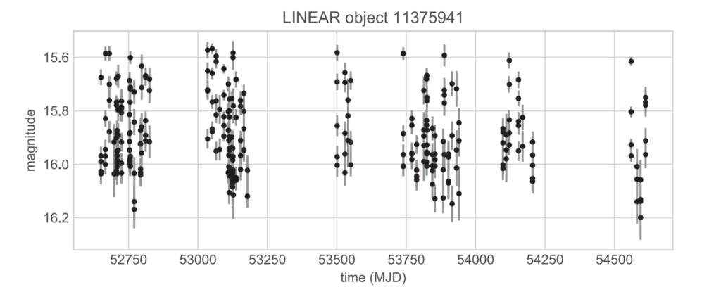
Many astronomers are interested in finding periodic signals. For instance, we look for periodic radial velocity variations to find exoplanets, and we look for periodic radio pulses to find pulsars. Often, these periodicities aren’t easy to see just by eye. For example, can you spot any periodicities in Fig. 1? Although there are several different approaches you could use, today’s paper discusses the most widely used method: the Lomb-Scargle (LS) periodogram. It can be used to find periodic, sinusoidal patterns in unevenly sampled data, and its approach is based on Fourier transforms.
Fourier transforms as the basis
You can think of a Fourier transform (FT) as an equation that can break a signal up into the different frequencies that make it up, like separating a chord into individual notes. The inverse scenario might be more intuitive: you can combine individual musical notes to build up a chord, in which case you effectively apply an inverse Fourier transform on all of your notes.
In the inverse FT, you thus combine sinusoids of different frequencies (i.e. your musical notes) to replicate a more complex signal (your chord). See also a visual example in Fig. 2, where we combine multiple sinusoids, shown in green, to recreate a signal shown in red. All of these sinusoids have a different frequency, as shown in the bottom panel.
In short, we can use FTs to convert our data into its underlying frequencies. Because frequency and period are inversely related, identifying a frequency is equivalent to identifying a periodicity!
A periodogram is calculated by taking the squared magnitude of the FT of your observations, from which we get a signal power at each frequency. You would expect this periodogram to tell you directly what the underlying frequencies are in your signal. However, things are slightly less straightforward when you consider that real observations are incomplete signals: we uncover pieces of a signal during observation, but that signal is lost when our telescope is, for example, observing another target or when the sun comes up.
How observing windows affect your periodogram
We can represent the times at which we are observing as a window function, such as shown in Fig. 3 (left). The window function is often a series of delta functions (at least, for short-duration observations). As you can see, what we actually end up observing is a product of the true signal and our window function. The right-hand panels show what our signal, window function, and resulting observations look like after applying a FT. These panels now relate to each other via a convolution instead of a product.
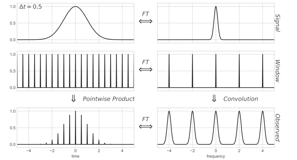
Our periodogram is therefore not a direct FT of the true signal that we are trying to discover, but is instead convolved with the window function. You can therefore think of the periodogram as nothing more than an estimate of the true signal’s frequency. The periodogram might not do a great job at finding the true frequency at all! For instance, compare the top right panel in Fig. 3, which would be the frequency signal you’re trying to look for, and the bottom right panel in Fig. 3, which would be the periodogram you actually obtain.
By taking a decent amount of observations, you can often manage to uncover the true frequency from your periodogram, but other strange things can also happen…
Lessons from 55 Cancri e
Let’s look at the real-world example of 55 Cancri e. This planet was discovered through radial velocities, which showed a very large peak at P = 2.808 days (see Fig. 4), interpreted to be the planet orbital period. However, transit observations later confirmed that the true orbital period of the planet was in fact 0.7 days! This very short orbital period makes 55 Cancri e famous for being an incredibly hot lava-world.
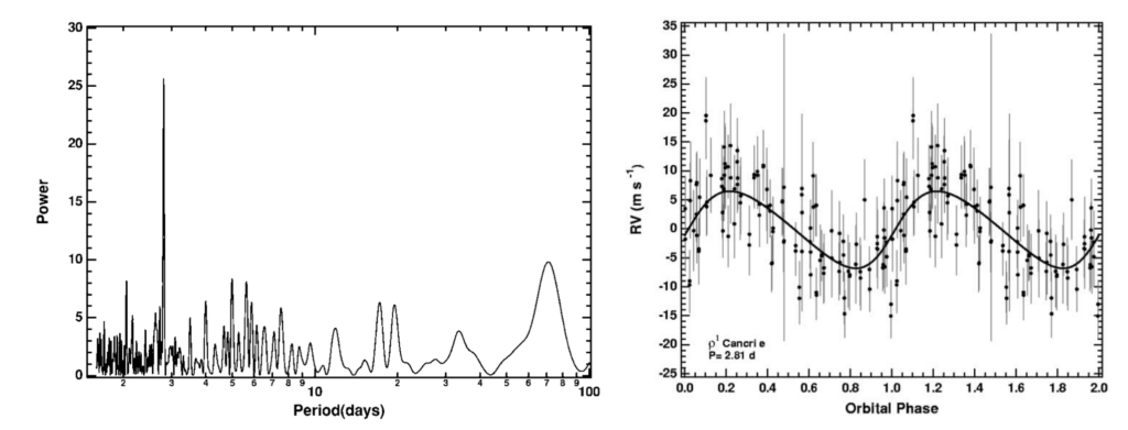
Remember, the periodogram is just an estimator of the true signal frequency. In this case, the periodogram is heavily influenced by day/night observing constraints. Because the observations only take place at night, the window function will be strongly periodic at a 1-day frequency. If we then combine the true 0.7-day planet signal with the 1-day periodic window function, we obtain a false-but-very-convincing 2.808-day signal. Such signals are often referred to as aliases.
Moral of the story?
The story of 55 Cancri e shows how the largest periodogram peak can’t immediately be trusted as the true frequency of your signal. Disentangling the true frequency signal from your periodogram requires a little bit more analysis and involves carefully inspecting your window function.
Today’s paper provides a list of recommendations to guide you through your periodogram analysis. So if you ever need a periodogram, check out today’s paper!
Astrobite edited by Julie Kiel Holm
Featured image credit: Altered from Jacob T. VanderPlas