- Title: Data analysis recipes: Fitting a model to data
- Authors: David W. Hogg, Jo Bovy, Dustin Lang
- Also see a lecture given by David Hogg at MPIA courtesy a series of YouTube clips starting here.
As astronomers, we find ourselves in a position to collaborate closely with other departments. The most obvious of these is physics, but the others include statistics, computer science, atmospheric science, geology, and engineering. Many astronomers are aware that sometimes we tend to forget the importance of understanding these subjects more deeply on our quest to understand the universe. Cue David Hogg et al. to remind everyone that fitting a line PROPERLY to data requires us to pull more out of our statistics toolbox than the trusty weighted least squares (WLS) fit. In fact, we may need to reach into a different toolbox all together.
So under what circumstances is using WLS the right thing to do? Hogg lists four requirements: 1) The errors are Gaussian; 2) You know your errors exactly; 3) Assume your errors are only in the y-direction (or x errors are negligible compared to y errors); 4) The data do come from a straight line (no intrinsic scatter). Your goal, of course, is to minimize an objective function χ2 which is the total squared error scaled by the uncertainties. So what’s the problem? Well, in astrophysics, rarely are all four of these conditions satisfied, and most likely, not a single one of them is satisfied. (1) can often be assumed, but is rarely exactly true, (2) is probably never true given that the errors on your errors are 4th moments and Hogg argues you never have enough data to calculate them, (3) occurs only in select scenarios like time of observation vs. position (time has a much smaller error bar than position), and (4) is also rarely true, usually astronomers talk about relations not linear laws.
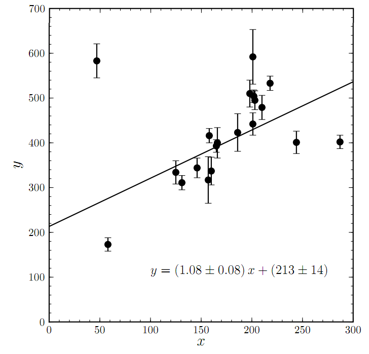
Well known techniques like "sigma-clipping" can rid you of pesky outliers and improve a bad fit like the one shown here. But Hogg argues the more responsible and scientific thing to do is model your bad points just as you do the points that belong.
The WLS procedure also runs into an additional problem when faced with outliers. There are many techniques for dealing with outliers, but one of the most widely used is called sigma clipping. For those of you unfamiliar, sigma clipping goes something like this. You have a data set which you have fit a line to, however there are points which lie way off the fit (or more than a certain amount, say 3.5 standard deviations (sigma)). So you remove all points greater than this distance from your fit and re-analyze the fit. Then repeat this procedure until you have converged on some data set (i.e. no more points are being excluded). This process works great, but Hogg argues that this is not science. He points out that sigma clipping does not optimize an objective function, and therefore cannot be compared in any reasonable way to another line fit by another procedure to the data. There are also other issues such as there is no guarantee it will converge! Oops!
So what to do? Well, there is a way to objectively reject bad data points. We can model them! However, to the chagrin of some, this requires we become Bayesian (Bayesian refers to statisticians who use methods made famous by Reverend Thomas Bayes). One way to do this is to use a mixture model where we assume the data comes from some combination of the actual model (the line) and some bad model (which you choose). But WAIT! You don’t know anything about your bad data so how can you justify a model for it? Well, by assuming something like a Gaussian for the bad model, the power of this does not come from actually being accurate, rather the power comes from simply modeling. By modeling instead of something like sigma clipping, you can marginalize over (integrate over) the parameters in the posterior probability distribution function you don’t care about (like the bad data) and optimize objectively. The way to do this is by using the Markov-Chain Monte-Carlo (MCMC) technique.
MCMC is a rather deep subject and for sake of space I will defer to literature. In summary, it is an algorithm that samples your parameter space to give you a measure of your posterior probability distribution without needing to test the likelihood at every point in your n-d parameter space. The amazing thing about it is that by simply projecting your sample into the parameter spaces you want, you have effectively marginalized over the other parameters. Very cool! Now, it is unfortunate that all this requires us to specify prior probabilities on our data, and this is definitely a cause for concern for many scientists. However, considering the alternative is important, that is, assuming those four things listed at the beginning are true. The priors we assign may not be completely accurate, but Hogg argues that using them is a far lesser crime than being ignorant of your assumptions. In the case of using priors, at least you are able to specify everything you are assuming about the problem, and others can challenge them.
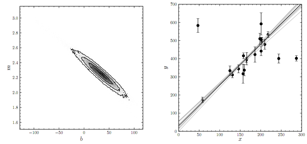
On the left is a sampling approximation to the posterior probability distribution that has been marginalized over the bad points. On the right, Hogg shows the maximum a posteriori (or MAP) fit and a sampling of other fits.
I encourage you to read both the paper posted to arxiv and watch his lecture which exists as a series of YouTube videos starting with this one. He also discusses other topics in both including different uncertainties, uncertainties in x and y (very important to watch/read), and intrinsic scatter which I may return to in another astrobite. Regardless of how you feel about Bayesian stats, Hogg reminds us that even simple analyzing procedures like fitting a line to data can be a much richer subject than you are taught, and trusting a one-size-fits-all procedure like weighted least squares should be carefully considered before proceeding. So check out a book on statistics from your university library, take a class on more modern statistical techniques, or attend an astrostatistics workshop and broaden your knowledge on a subject you will be happy to know well. David Hogg, your advisor, the referee of your next paper, and the astronomical community will thank you!


A really good paper that summarizes how to implement MCMC in an astronomical context is Ford 2005 (ApJ vol 129 issue 3).