Checking up on Circumstellar CO

Title: The Photodissociation of CO in Circumstellar Envelopes

Authors: M. A. T. Groenewegen

First Author’s Institution: Koninklijke Sterrenwacht van België, Ringlaan 3, B–1180 Brussels, Belgium

Status: Astronomy & Astrophysics in Press [open access]

The stuff surrounding stars

We can all acknowledge that stars are some of the coolest objects (figuratively speaking) in the Milky Way galaxy.  But today we consider something even cooler (literally speaking): the envelopes of certain stars.

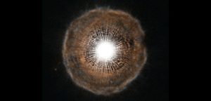
Figure 1: A spectacular Hubble image of a star near the end of its lifespan, spewing out shells of gas. Image Credit: [ESA/Hubble, NASA and H. Olofsson (Onsala Space Observatory)].

Today’s astrobite looks at modeling carbon monoxide (aka, CO) in the envelopes, or layers of shells of gas, around evolved stars (hence the name circumstellar envelopes; check out this astrobite for some more discussion!).  CO is pretty infamous enough here on Earth, but it’s also famous in space for an entirely different reason: it’s actually the second-most abundant known molecule (after molecular hydrogen, H₂).  CO plays a crucial role in the envelopes surrounding evolved stars – and so understanding how CO is distributed in these circumstellar envelopes can help us understand the chemistry of these systems overall.

Back in 1988, a certain research group (Mamon et al. 1988) laid out a model that described the CO distribution of these circumstellar envelopes using just two parameters – an aptly-named “two-parameter model”, in short.  They determined the values of those two parameters for different systems, such as for envelopes with different expansion velocities and with different mass-loss rates.  Then the group published their determined parameters for these different systems in a nifty table.  Other research groups built upon this table of parameters and the two-parameter model, and used the results to estimate the size of CO envelopes about evolved stars.

But 1988 was nearly 30 years ago (how time flies!) – and a lot’s changed in the past 30 years.  For example, there are now detailed ways to deal with shielding, which is the phenomenon where molecules in the outer layers of an envelope can be shielded from the central star’s light by molecules in the inner layers (just like how crowded front rows can block back rows in an outdoor theater).  There are also new ways to solve the problem in two dimensions numerically now, rather than relying on analytical approximations to simplify the problem as the 1988 group did.  And it’s also a lot clearer nowadays that external radiation coming from the surrounding interstellar space – not just from the central star – is an important factor for these envelopes as well.

The author of today’s astrobite set out to essentially update the work from 1988, taking into account the past 30 years of research and innovation, and provide a brand-new table of parameters for everyone to use.

An iterative approach

Today’s author took a combined analytical and numerical approach to calculate a new table of parameter values.  They used the analytical two-parameter model from the 1988 group, which has the following form:

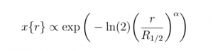
Here, r is the radius, x(r) is a variable that describes the CO profile at radius r, exp is exponential and ln is natural log, and α and R_1/2 are the two parameters that we want to know.  The author then made some key assumptions: they assumed that the system was spherically symmetric and uniform, with a constant speed of expansion.  These simplifications allowed them to calculate the CO profile with the following numerical approach:

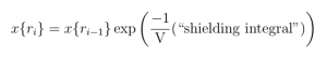
Now, we have that x(r_i) is the CO profile at radius r_i, x(r_i-1) is the CO profile one increment smaller in radius, and thus one step closer to the central star (like how stepping down a stair brings you closer to the ground floor).  V is the expansion velocity, and the “shielding integral” is a term that, among other things, takes care of the effect of shielding mentioned earlier.

Wrapped up in the “shielding integral” term are the very two parameters, α and R_1/2, that come up in the 1988 two-parameter model!  So in order to figure out the values of the two parameters for a given system, the author essentially iterated back and forth between the analytic and the numeric approach:

1. Start with values for α and R_1/2
2. Use the α and R_1/2 to calculate the “shielding integral” term
3. Plug into the numerical equation and calculate x(r_i) for every step in radius
4. Piece together the results from Step 3 at every radius to form a full distribution across the envelope
5. Fit the two-parameter equation to the pieced-together numerical results from Step 4, thus getting new values for α and R_1/2
6. Repeat until basically no change in α and R_1/2 between Step 1 and Step 5

They calculated α and R_1/2 in this way for a number of systems with different characteristics.  For example, they considered systems immersed in different interstellar radiation field strengths.  They also looked at systems with different mass-loss rates and expansion velocities.  They summarized all of these different system characteristics, and their resulting parameter values, in a new nifty table, mirroring the table published so many years ago by the 1988 group.

Then… and now

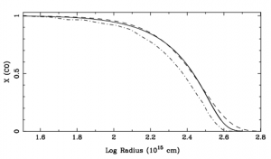
Figure 2: A plot of the CO profile (y-axis) against the log of the radius (x-axis) for one system considered. The solid line is from this astrobite’s numerical work, while the dashed line is the profile from the associated two-parameter model. The dotted-dashed line is the profile based on the 1988 work for comparison. Note the differences at larger radii! Figure 2 in the paper.

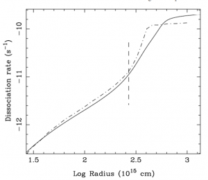
Figure 3: A plot of dissociation rate (y-axis), a quantity that relates to shielding, against the log of the radius (x-axis) for a particular system. The solid line is from this astrobite’s work, while the dotted-dashed line is based on the 1988 work.  Again, note the differences at larger radii!  The vertical line indicates the R1/2 value for this model. Figure 1 in the paper.

Figures 1 and 2 compare example results from today’s astrobite to results based on the 1988 group.  In both figures, we can see differences in the two approaches, particularly at large radii.  And so this astrobite encourages readers to interpolate directly from its new table of updated values for future CO envelope modeling.

This is a timely update, too!  The snazzy new interferometer known as the Atacama Large Millimeter/submillimeter Array (aka, ALMA) has been pouring out oodles of gorgeous higher-resolution data.  It can resolve the extent of CO envelopes around evolved nearby stars better than ever before.  So with the work of today’s astrobite, we can lay down a new and improved theoretical base for these envelopes, so that we can not only predict what we’ll see in the observations, but also better interpret what they have in store.