Title: Primordial Black Holes from Inflation and Quantum Diffusion
Authors: Matteo Biagetti, Gabriele Franciolini, Alex Kehagias and Antonio Riotto
First Author’s Institution: Insitute of Physics, Universiteit van Amsterdam, Science Park 1098XH Amsterdam, The Netherlands
Status: open access on arXiv
Primordial black holes are on the cosmologist community’s most wanted list because they make promising dark matter candidates (see here for an astrobite that explains why). They’ve risen through the ranks recently because the gravitational waves that LIGO detected came from merging black holes. The black holes were relatively light and could have formed early enough to have been primordial.
This tantalising detection means that a lot of effort has been put into finding models of the early universe that produce enough black holes to make up all of the dark matter. Today’s authors have shown that we all need to be extra careful with how we come up with these models – it turns out that pesky quantum effects can mess around with the number of primordial black holes that could be around today.
Overdense vs underdense
In order for primordial black holes to have formed in the early universe, there need to have been lots of regions dense enough to collapse. Overdensities were produced while the universe was in an initial phase of rapid expansion known as inflation. Quantum uncertainties allowed some patches of space to expand more than the average, meaning they were less dense, whilst some patches didn’t get to expand as much and were therefore more dense.
We measure the level of overdensity in patches of different sizes with the primordial power spectrum. If there are lots of overdense patches of a particular size, then the amplitude of the power spectrum at that scale is larger. So, if there were regions dense enough to form black holes at a certain scale, there would be a peak in the power spectrum at that scale. In practice we actually measure the Fourier transform of the primordial densities, so the power spectrum is a function of 1 over the physical size of the patches – think wavenumber instead of wavelength.
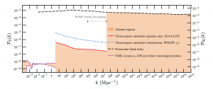
Figure 1: The power spectrum as a function of scale. The orange region represents allowed values according to current observational constraints. Large physical sizes correspond to small values of k to the left of the plot where the strongest constraints can be found. Figure from Bringmann et al. 2011.
The orange region in figure 1 shows the currently allowed region for the primordial power spectrum. Observations have done well to constrain the power to around \(10^{-9}\) on small k-values, which correspond to large physical patches. However, on smaller physical patches (larger k-values) the constraints are a lot weaker. The aim in terms of primordial black holes is to fit a peak somewhere to the right-hand side of this plot – e.g. if LIGO detected primordial black holes, there would be a peak at about k=\(10^{5.5}{\rm Mpc^{-1}}\).
The inflaton and how it rolls
During inflation, particles like photons and baryons hadn’t formed yet, so we call whatever was around to drive this phase of rapid expansion the inflaton. How inflation plays out depends on how the inflaton’s kinetic and potential energy evolve. We can picture this as a ball rolling down a hill, where the hill describes the potential, and how fast it’s rolling describes its kinetic energy. When the ball reaches the bottom, inflation ends and the inflaton decays into the things we see today like matter and radiation.
Slow-roll inflation (a mathsy but good explanation here) is the simplest model we have. The inflaton rolls (you guessed it) slowly down the potential and this produces an almost flat power spectrum. This matches the flat section of the power spectrum that we’ve measured well on the left-hand side of figure 1. We characterize slow-roll models with the parameter \(\epsilon\) which tracks the ‘velocity’ that the inflaton is rolling down the potential, and is inversely proportional to the amplitude of the power spectrum: \(\mathcal{P}\sim1/\epsilon\).
If \(\epsilon\) is small and constant then we’re safely in the slow-roll category and we can make lots of nice approximations that make the calculations easier. However, for primordial black holes, we don’t want flat the whole way along– we want a peak in the power spectrum.
If we can make \(\epsilon\) decrease rapidly, the power spectrum will grow rapidly and we’ll be in the money with a primordial-black-hole-friendly peak. If \(\epsilon\) has decreased a lot, the inflaton will roll very slowly, and the potential will be very flat – we’ll enter an ultra slow-roll regime.
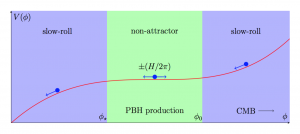
Figure 2: The red line represents the potential, and the blue dot represents the inflaton rolling through the three different phases. Figure from today’s paper.
Today’s authors model this scenario with an initial slow-roll regime, followed by a flat region in the potential that induces an ultra-slow-roll phase, followed by a final slow-roll phase. This is illustrated in figure 2. The exact details of the transitions between the phases characterize the peak, and the underlying model has to be engineered carefully if the peak is to guarantee black holes of the right mass and of the right number.
Figure 3 shows a peak produced by a specific model that the authors choose. Imagine lining up the red peak in figure 3 at the scale you want your black holes to form on figure 1, and lining up the flat section on the left with the well constrained scales at small k.
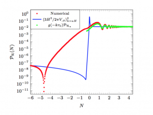
Figure 3: The power spectrum prediction for a specific model in today’s paper. Analytical calculations that the authors did only allowed them to study the ultra slow roll phase shown by the green line, whilst numerical calculations give the full picture for a complicated transition between phases, shown by the red line. [latex]N\sim\log{k}[/latex]. Figure from today’s paper.
Quantum kicks
Now that we’ve got a peak, we can worry about quantum effects again. During ultra-slow-roll, our slow-roll approximations no longer work, and quantum effects mean that the velocity of the inflaton (which is roughly \(\sqrt{\epsilon}\)) can be shifted around the classical average in different patches of the universe. This means that you can’t be sure of the final amplitude of the power spectrum since this depends on \(\epsilon\). The authors find a condition which ensures quantum effects don’t mess around with the power spectrum too much, and show that it’s violated by some inflation models that are able to produce an interesting number of primordial black holes. Since the number of black holes produced is related to the power spectrum amplitude by a logarithm, even if the power spectrum only changes by a little, the number of black holes produced can vary hugely.
Today’s paper points out how fragile the process of producing primordial black holes can be. Being able to accurately predict the outcome of a model is really important so that we know what to go out and look for. That’s why exploring a model’s weird and wonderful finer details, as today’s authors have done, will ultimately help to constrain our ideas on how inflation happened, and what got left behind.
Author