Brown Dwarf Weather Forecast: Cloudy or Clear Skies?

Title: Retrieval of SDSS J1416+1348AB

Authors: Eileen Gonzales, Ben Burningham, Jackie Faherty, Colleen Cleary, Channon Visscher, Mark Marley, Roxana Lupu, Richard Freedman

First Author’s Institution:Department of Astronomy and Carl Sagan Institute, Cornell University, 122 Sciences Drive, Ithaca, NY, USA

Status: Preprint on arXiv

In the space between stars and planets lives a class of astronomical objects known as brown dwarfs. Too massive to be planets (~75 times more massive than Jupiter!) but not massive and hot enough to fuse hydrogen like our Sun, these objects are nevertheless classified like stars with spectral types—in other words, by the molecules we detect in their emission lines. Depending on their spectral type, dwarfs can be classified as one of the subdwarf types, usually marked by a letter, indicating the types and abundances of metals we detect in their atmospheres. These abundances can reveal clues about the process by which brown dwarfs are formed, which in turn informs our understanding of how planets and stars come to be. 

In today’s paper, the authors consider a binary system of two brown dwarfs of different spectral subtypes, and in particular the dwarfs’ atmospheres. First discovered by SDSS and lovingly called SDSS J14162408+1348263AB (but we’ll follow the authors in calling it J1416AB), this system is unique because it is the only known binary of subdwarfs with the spectral types L and T (see Figure 1 for some general information about brown dwarf spectral types). This means the two dwarfs have both different temperatures and different chemical composition of their atmospheres while living in the same neighborhood in space. In analyzing this binary system, the authors can compare each of the dwarfs and make predictions about what their atmospheres look like, what molecules are present, and whether they were created and evolved together. In addition, they can test out different atmospheric models on the existing observational data of these objects to find the one best suited to low-metallicity subwarfs’s atmospheres.

Figure 1. An illustration of brown dwarf spectral types and how they compare to Jupiter and our Sun. Both L and T subdwarfs are distinguished by absorption lines of metal hydrides (for instance, FeH) and weak or absent metal oxides (like TiO and CO). Image from WikiCommons.

Finding the best atmosphere models

Today’s paper uses something a code called Brewster, which is modified to be specifically well suited for low-metallicity atmospheres (like the ones in L and T type dwarfs). The first step in modelling the atmosphere is setting up a relationship between pressure and temperature of the atmosphere based on the gasses present in each layer. The authors subdivide the atmospheres into 65 layers constituting three zones: the bottom two zones have an exponential relationship between temperature and pressure, and the top zone is isothermal, meaning that the temperature stays constant. They also look for abundances of the elements most present in the spectra of the two dwarfs (including water, carbon monoxide, methane, and more). Finally, the authors model the cloud cover in the atmosphere by considering the opacity of each of the atmospheric layers. The opacity of the layers is set by the presence of alkali atoms (specifically, sodium and potassium) in the atmosphere.

Once they know what parameters they’re interested in retrieving, as well as some prior information about the system from observations (for instance, the total amount of any one gas if not how it’s distributed in the atmosphere), the authors can run a lot of simulations of their models with different parameters until they find the winning model and parameters which best match the data.

What’s the weather like on brown dwarfs?

The authors performed individual analysis on each of the members of the binary: J1416A (the L dwarf) and J1416B (the T dwarf). The paper contains thorough analyses for several types of cloud models and two different alkali opacity values; for the purposes of keeping this summary a bite rather than a meal, we’ll only show the results of the best fit models for each of the dwarfs. 

In the case of J1416A, the best fit is achieved with a cloud model called the power-law deck cloud model (see Figure 2). In the case of J1416B, a cloudless model provides the best fit, which is consistent with previous literature for this particular object (see Figure 3). When coupled with a particular choice of alkali opacity numbers from previous literature, only these two models produce abundances of alkali atoms expected for the system from observational data. Finally, these model choices yield approximately the same metallicities for each of the dwarfs (about the same as our Sun!), suggesting that the pair both formed and evolved together!

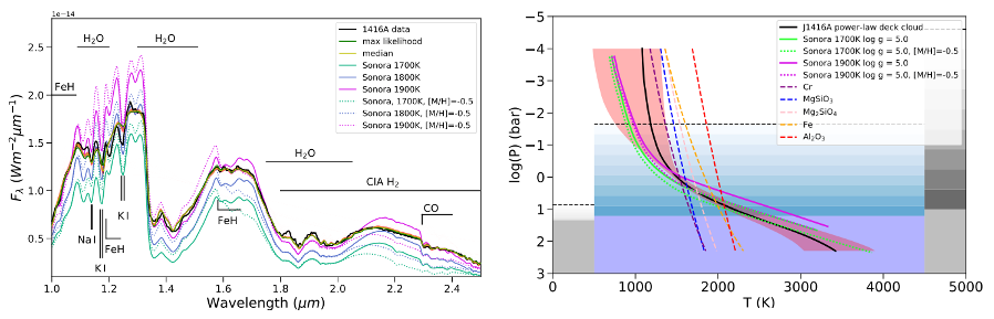
Figure 2. Parameters for J1416A. On the left is a plot of the energy flux per meter squared for each wavelength shown, with atmospheric element names written next to their corresponding spectral lines. The black line is the spectral data for the object, with the maximum likelihood and median model shown in the two greens. In addition, a cloudless atmosphere model called Sonora is shown in teal, purple, and magenta for three different temperatures and two different metalicities. On the right is a plot of the Pressure-Temperature Profile for a choice of cloud model as optimized by the model (in black), and of the Sonora models introduced on the left. The condensation lines of the indicated molecules are shown in colored dashed blue lines indicate the median cloud deck cover, with the purple showing where the atmosphere becomes completely optically thick. Note that the Sonora cloudless lines are similar to the authors’ model, except in the top isothermal layer of the atmosphere, indicating that J1416A is probably cloudy. Figures 10(a) and 7(a) in the paper.

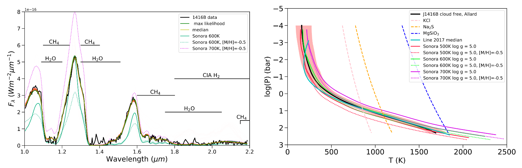
Figure 3. Parameters for J1416B. As above, on the left is a plot of the energy flux per meter squared for each wavelength shown, with atmospheric element names written next to their corresponding spectral lines, along with Sonora cloudless models for appropriate temperatures and two types of metallicities. On the right is a plot of the Pressure-Temperature Profile for a choice of cloudless model as constrained by the authors (in black), and of the Sonora models introduced on the left (as well as one from another paper by Line et al.). Again, the condensation lines of the indicated molecules are shown in colored dashed lines. Because both models here are cloudless, there’s an even better match between the authors’ and the Sonora model than for J1416A, as well as a good match with the results from Line et al. Figures 13(a) and 11(a) in the paper.

Even more atmospheres!

In today’s paper, the authors took a deep dive into the nuances of modelling two subdwarfs’ atmospheres, including Pressure-Temperature Profile models, different opacity numbers, and cloud cover models. Using the J1416AB binary to cut their models’ teeth, they can confidently model both cloudy and cloud-free atmospheres. The next step is to use the modelling tools developed in this paper specifically for low metallicity subdwarfs to analyze a larger sample of astronomical objects to understand the nuances of subdwarf atmospheres, as well as atmospheres of sources with similar spectral types and temperatures.

Astrobite edited by: Alex Pizzuto 

Featured image credit: Ann Field (STScI) / Univ. of Wisconsin, Madison