Title: Physical-based scattering model for Titan: Integrating Cassini microwave data (active and passive)
Authors: F. Grings, M. Franco, M.G. Spagnuolo, M.A. Janssen, R. Lorenz
First Author’s Institution: Instituto de Astronomía y Física del Espacio (UBA-CONICET), Ciudad Universitaria, Buenos Aires, Argentina
Status: Published in Icarus [closed access]
Ingredients for understanding Titan
Even after the Cassini mission spent 13 years orbiting Saturn and performing dozens of flybys of its largest moon, Titan, many questions remain. Part of the reason Titan has been reluctant to share its secrets is the great thickness of its atmosphere, which blocks most wavelengths of light that the human eye can see. Fortunately, Cassini was equipped with a radar instrument specifically to deal with this issue! The longer wavelengths transmitted and received by this device pierced Titan’s deep haze and revealed dramatic landforms not unlike those on Earth: mountains, lakes, river valleys, dunes, and vast plains—all likely composed of various ices, liquid hydrocarbons, and exotic organic compounds like tholins, kept at a crisp 95 Kelvin (-289 °F or -187 °C).
Despite radar’s great capabilities for observing Titan, making a precise interpretation of the data is often challenging. At the microwave wavelengths of the Cassini radar instrument (λ ~ 2.2 cm), the measured intensity is a function of many attributes that include both the angle of the radar beam relative to the ground as well as the dielectric and geometric properties of the surface. The dielectric constant of a material is essentially its reflectivity at microwave wavelengths, which is dependent on the composition. Geometric properties include the roughness of the surface relative to the imaging wavelength, so a surface on Titan that is very rough at ~2 cm (covered in cobbles and pebbles, perhaps) will return greater microwave intensity than a smoother surface (like a sandy beach).
The synthetic aperture radar mode on Cassini’s radar instrument pinged the surface to produce images measuring the radar backscatter, and the passive radiometry mode collected microwave light emitted from the surface. The resulting values, the backscattering coefficient (σ0) and the microwave emissivity (ε), are linked by Kirchhoff’s Law of thermal radiation—essentially, “good emitters are good absorbers,” (and good absorbers are bad reflectors!). By studying both properties in tandem, one can better constrain the information they suggest about Titan’s surface. Such a tactic is helpful, considering Titan has given us some rather anomalous radar data.
A new recipe to explain Titan radar
Several studies have incorporated various scattering models to explain the very high radar backscatter from Titan while maintaining the low dielectric constant expected for Titan’s icy, organic-rich surface. The authors of today’s bite argue that whereas previous models include inconsistent assumptions about the surface that aren’t based in reality, their proposed model is physically consistent while incorporating both radar backscatter and emissivity to maximize accuracy. Subsurface scattering has typically been invoked to explain the unusually bright radar backscatter from Titan, and is incorporated into the proposed model in a relatively simple way. Since radar tends to reflect from interfaces where there is a change in the dielectric properties (e.g., air vs ground, sea vs seafloor, etc.), the model uses two layers (see Figure 1) so that microwaves can bounce between these subsurface layers multiple times (AKA volume scatter) before finally shooting back to the radar instrument. In the model, σ0 and ε are dependent on the angle of the radar beam hitting the surface and a handful surface properties like the roughness, dielectric properties, and thickness of the layers. If they can find the right combination of model inputs that produce outputs matching the Cassini observations, they can say with some probability what the properties of the surface there are.
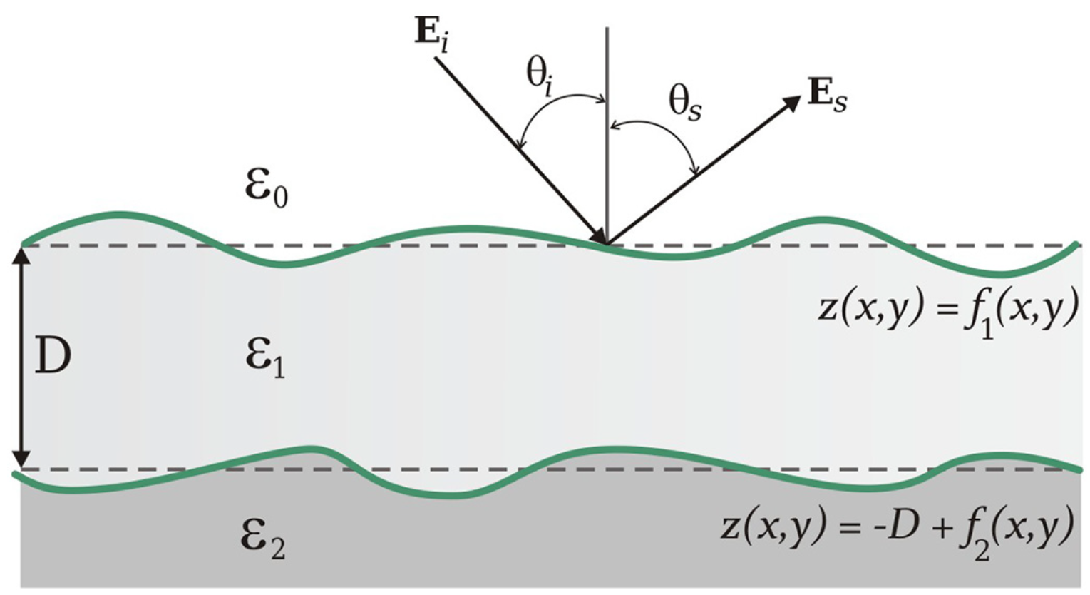
Figure 1 – Diagram illustrating the two-layer model utilized by today’s paper. The dielectric constants ε0, ε1, and ε2 represent that of the air, upper surface layer, and lower subsurface layer, respectively. The thickness of the upper surface layer is represented by D. Inbound/outbound radar beams and their reflection angles are represented by E and θ, respectively. The function z(x,y) describes the roughness of the interfaces at the top of the surface layer and between the surface and subsurface layers. Figure 5 from today’s paper.
The authors selected a region on Titan where they could study different types of terrain across multiple overlapping datasets. Incorporating a set of emissivity data with criss-crossing images of radar backscatter from three different Titan flybys allowed them to see how the terrains scatter light at various angles, a behavior that can suggest specific dielectric and geometric properties. In essentially a small-scale version of previous Titan mapping efforts, four different terrain units (see Figure 2) were mapped. Each terrain has a different combination of radar backscatter and microwave emissivity that the model needs to be able to explain based on reasonable surface properties.
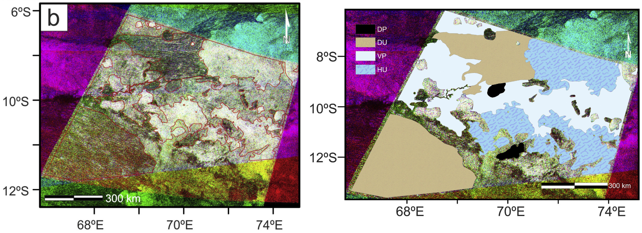
Figure 2 – Maps of the study region on Titan showing the four different terrain units in a combined radar image (left) and with the mapped units colorized for clarity (right). The terrain units are hummocky (HU), variable-featured plains (VP), dunes (DU), and dark irregular plains (DP). The background in each map is an RGB combination of the three radar swaths where each is assigned either the color red, green, or blue so that where they overlap the highest radar backscatter if bright white and lowest is dark black. From Figures 2 and 3 in today’s paper.
The observed mean radar backscatter and emissivity for each unit across the variously-angled radar images can be seen in Figure 3. Employing their model to match these observed values, the authors first tested the sensitivity of the expected radar signal to changes in various surface properties and found the expected trends of higher σ0 with rougher surfaces and so on. Interestingly, increasing the layer thickness D will alternate between increasing and decreasing σ0, due to constructive and deconstructive interference as the bouncing radar waves go in and out of sync. By adjusting such parameters, the model found reasonable surface properties that for the first time can simultaneously explain the anomalous radar backscatter and emissivity values recorded by Cassini.
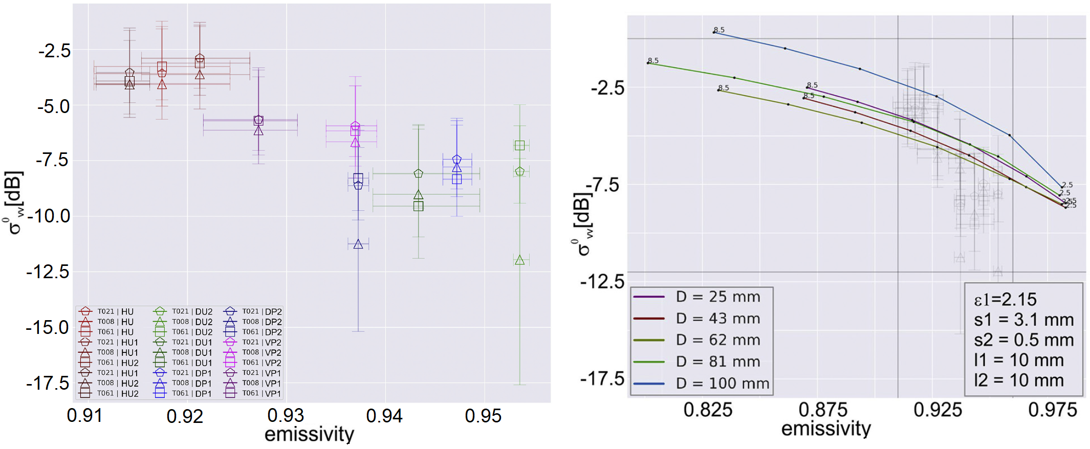
Figure 3 – The plot on the left shows the observed radar backscatter (σ0) and emissivity (ε) values for different terrain units across in each radar image. Different subunits are plotted in slightly different colors but depict hummocky units (HU) in red, dune units (DU) in green, dark irregular plains units (DP) in blue and variable-featured plains (VP) in purple. Note the apparent “trade-off” between σ0 and ε as expected from Kirchhoff’s Law. The plot on the right depicts these same observed values in a light gray for reference, but also plots one iteration of the model that illustrates how different surface layer thicknesses (D) change the output while all other values are held constant. Modified from Figures 4 and 6 in today’s paper.
The icing on top (with ice on the bottom!)
Reassuringly, the modeled surface properties are consistent with previous work, and can even more tightly constrain some relatively uncertain parameters. The modeled results for most units indicate a smooth upper layer of material with low dielectric constant, a couple feet or less thick, atop material of higher dielectric constant. For example, the dune units may represent an upper layer of tholin-like organics deposited from the atmosphere, on top of a lower layer that is a more ice-rich, rougher mixture of materials. Roughnesses from the model are generally low overall, but may be consistent with the size and distribution of low, wind-made ripples of sand (~1 mm tall with ~10 cm spacing), whereas previous studies disagree on whether such forms could actually develop on Titan.
Innovative models such as that in today’s paper inherently involve a fair amount of error due to the necessary assumptions, unknowns, and non-unique solutions. However, each iteration can bring us closer to developing an understanding of the reality of Titan’s surface. This two-layer model incorporates volume scattering to account for Titan’s radar backscatter and emissivity in a realistic manner. Future models will be able to build on this work to study the influence of even more detailed properties of the surface and subsurface to continue developing a better understanding of Titan and what future surface missions to this world can expect to encounter.
Astrobite edited by Wynn Jacobson-Galán
Featured image credit: Caitlyn de Wild and today’s paper