Title: A compositional link between rocky exoplanets and their host stars
Authors: Vardan Adibekyan, Caroline Dorn, Sérgio G. Sousa, Nuno C. Santos, Bertram Bitsch, Garik Israelian, Christoph Mordasini, Susana C. C. Barros, Elisa Delgado Mena, Olivier D. S. Demangeon, João P. Faria, Pedro Figuiera, Artur A. Hakobyan, Mahmoudreza Oshagh, Bárbara M. T. B. Soares, Masanobu Kunitomo, Yoichi Takeda, Emiliano Jofré, Romina Petrucci, and Eder Martioli
First Author’s Institution: Instituto de Astrofísica e Ciências do Espaço & Departamento de Física e Astronomia, Universidade do Porto, Porto, Portugal
Status: Published in Science [closed access]
Background
Though we don’t yet have a complete picture of planetary formation – especially for types of planets we don’t find in the Solar System – we do have a good idea of the overall process. It starts with a cloud of gas and dust somewhere in space. Turbulence will then cause clumps of mass to form within the cloud. When there’s enough mass, the clump will collapse in on itself due to gravity, heating up and forming a protostar. Over time, a disk forms around the protostar from the remaining gas and dust – the protoplanetary disk. Within that disk, more collisions occur, and dust grains clump together, eventually becoming protoplanets. Mass will continue to accrete onto the protostars and protoplanets, essentially meaning that the gas and dust “fall” onto the mass clumps, making them bigger. Eventually, the protostar grows into a main sequence star, and the protoplanets are either destroyed or become full-blown planets.
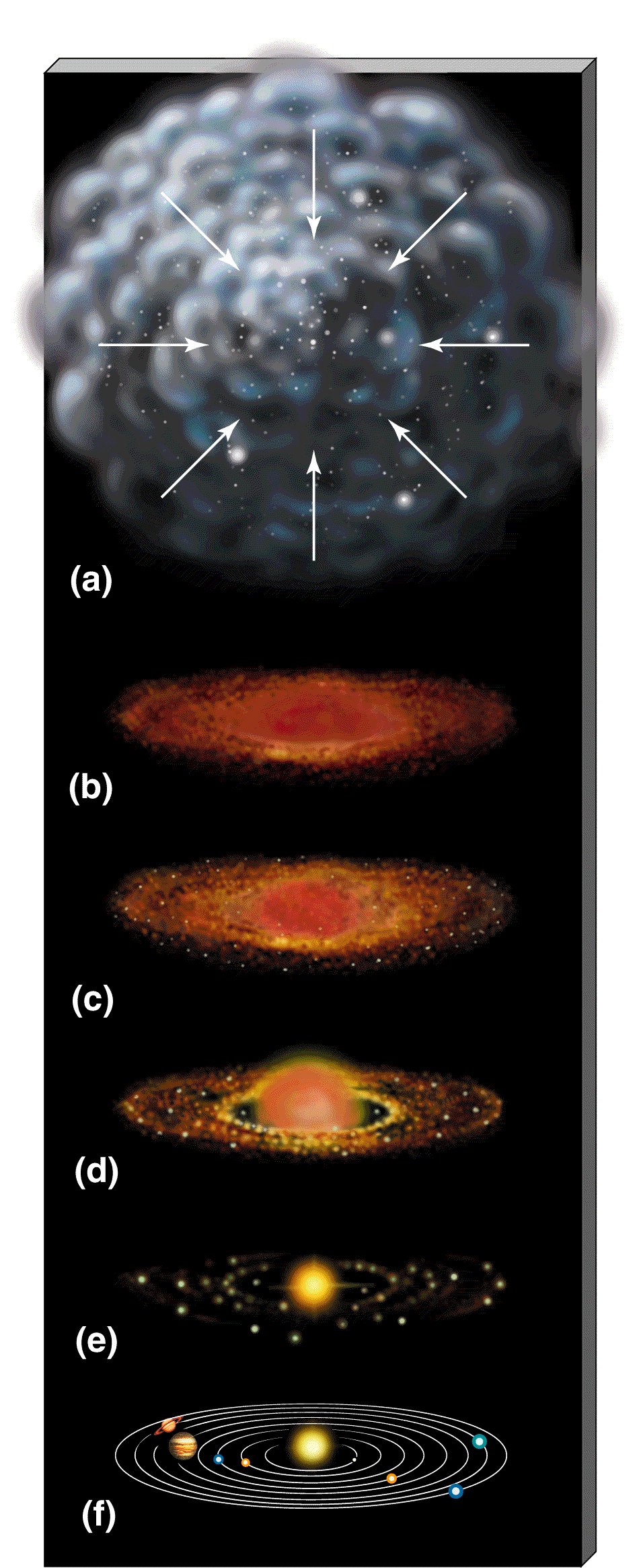
Figure 1: The steps of star and planet formation are shown here, as follows: a) the gas cloud collapses, b) the protostar begins to form, c) the protoplanetary disk forms around the protostar, d) material starts to clump together, forming protoplanets, e) the protoplanets have grown larger and the remaining gas and dust has dissipated, and f) the resulting system (in this case, the Solar System)
The chemical composition of the protoplanetary disk and the resulting planets can tell us important information about the formation mechanisms of the planets, as well as the potential characteristics of the planets. With current observational technology, we can’t always determine the composition of the planet itself. But, since this whole system originates from the same cloud of gas and dust, learning information about the chemical composition of the stars can also tell us information about the planets around them. We can do that relatively easily using stellar spectroscopy, since different elements present in a star or planet will emit and absorb different wavelengths of light in a spectrum.
Methods
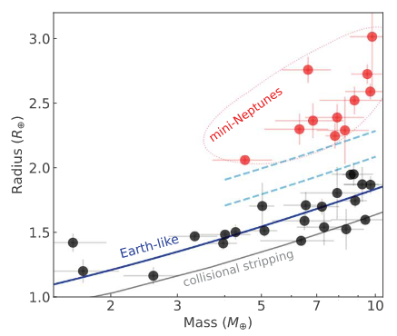
Today’s authors investigated 32 known exoplanets with masses M < 10 MEarth orbiting 27 different sun-like stars to find a correlation between terrestrial planet formation and the composition of planetary host stars. All 32 of the planets have known masses from radial velocity measurements and known radii from transit measurements. The authors plotted them on a mass-radius diagram and removed 10 planets that are likely mini-Neptunes from the sample (see Figure 2). They then determined the abundances of Mg, Si, and Fe – all major rock-forming elements – in the host stars using their spectra. Using pre-existing stellar composition models and these abundances, the authors estimate the iron abundance of the stars and protoplanetary disks relative to Mg and Si. Using the masses and radii of the planets and existing planetary interior models, they then estimate the iron abundance – again relative to Mg and Si – of the planets, independent of the star.
Results
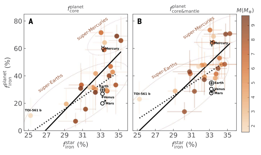
Figure 3 shows the results of plotting each planet’s resulting iron abundance versus its host star’s iron abundance. Indeed, we see a positive correlation between the iron abundance of these terrestrial planets and their host stars. Interestingly, the results suggest that five of the planets in the sample are likely “super-Mercuries”, planets which have similar compositions to Earth, but much higher masses relative to their radii, similar to Mercury in our solar system. All five super-Mercuries orbit stars with high iron-to-silicate ratios and high iron abundances, which suggests that the planets’ compositions may be related to their stellar and protoplanetary disk compositions. Under these conditions, more collisions would likely occur during the planet formation process, lending credence to the theory that Mercury and Mercury-like exoplanets were formed through collision processes. Though more data is needed on super-Mercury populations, this study could potentially be adding another piece to the puzzle of planet formation!
Astrobite edited by Katya Gozman
Featured image credit: ESO/L. Calçada
I had never thought of similarities in composition between planets & their host stars before. Thank you.