Paper Title: Predicting convective blueshift and radial-velocity dispersion due to granulation for FGK stars
Authors: S. Dalal, R. D. Haywood, A. Mortier, W.J. Chaplin, N. Meunier
First author institution: University of Exeter
Status: On ArXiv (open access)
New and better than ever spectrographs are finally in use at observatories around the world and this makes exoplanet-hunting astronomers excited to see what discoveries they will help reveal. These instruments are used to perform the radial velocity (RV) technique for discovering new exoplanets. The RV method works by measuring the Doppler shift of the star’s light from the motion of the star due to the planet orbiting it. To discover an Earth-twin planet, that is a one Earth mass planet orbiting a 1 solar mass star every 365 days, requires us to be able to measure a 10 cm/s velocity shift. That’s so tiny, it’s about the speed of some species of tortoises. At the dawn of the field of exoplanet research, measuring a signal this small was unthinkable: early instruments were only capable of measuring ~10 m/s, a whole 2 orders of magnitude larger than required! But in the 30 years of the field, we’ve learned how to build better spectrographs and now the newest fleet of instruments can measure as small as 30 cm/s. We’re getting close!
However, it’s not as straight-forward as it may seem. In an RV dataset, we hope to find signals that are produced by planets, but the host star can also produce signals (called stellar activity) that appear in our data. Unfortunately, signals from planets and signals from the host star often look exactly the same in our data and so it can be a challenge to determine exactly where your signal is coming from. If not careful, a stellar signal can be mis-identified as a planet (False Positive planet detection) or a planet signal can be mis-identified as a stellar signal (False Negative planet detection). Therefore, it’s very important to make sure a signal is properly accounted for. But to make matters worse, stellar induced signals come in many different flavors. Each flavor is due to a different physical phenomenon and therefore it exhibits in our data at different amplitudes and on different timescales.
In today’s paper, the authors explore one of these flavors of stellar activity: Convective Blueshift. First, let’s explore the background of the topic and break down the term.
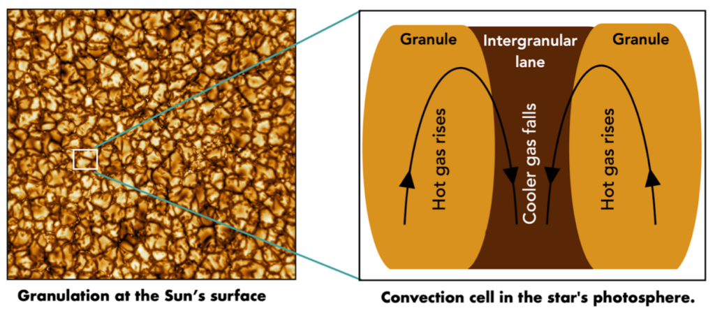
First “Convective”. Stars are not rigid, solid objects. Instead, they are balls of fluidly moving gas. Think of the surface of a star like a deep ocean, but instead of water, it’s a gas. In a star, the deeper you go into that gaseous ocean, the hotter it gets. However, just like in our own daily lives, hot air rises. This is what powers a hot air balloon, for example. So the hotter gas deep within the star wants to rise up to the surface of the star. As the hot gas moves up to the surface, it begins to cool down. When it reaches the surface and is cooled, now it wants to sink back down as new hot gas from below pushes up and displaces the cool gas downward. This is called convection. It’s the same idea that heats your food in a convection oven, which continually circulates newly heated hot air to keep the oven hot and push out the cooler air.
So as hot gas rises to the surface of the star, that bundle of gas is moving towards us here on Earth, see Figure 1. But the cooler gas that is displaced and moving downward into the star is moving away from us. So within a small area of the surface of the star, called a granule, we have some gas moving up aka towards us, or getting blueshifted, and other gas moving down aka away from us, or redshifted. At first we might guess that there is an equal amount of gas moving towards and away from us, so the blue and red shifts should cancel out. However, there is a trick. Hot gas is brighter than cool gas, so that hot gas moving towards us shows up more strongly in our measurements. Therefore we get a net blueshift in our data. Hence the name “Convective blueshift”.
Now let’s talk about today’s paper! The authors describe a new mathematical framework for modeling and predicting the extra stellar activity signal noise in an RV data set due to this convective blueshift phenomenon. They do this by first estimating the number of granules on the surface of the star by relating this value to the size (both mass and radius) of the star and its temperature. At this stage, the authors determine that cooler stars have more granules on average than hotter stars. Then they estimate the velocity of the hot gas rising in each of these granules by relating the speed to the temperature of the gas and the mass of the star. Together they provide a tidy expression for the estimate of the amplitude of the convective blueshift. From there, they relate these values to the RV scatter expected from this many granules contributing this average velocity.
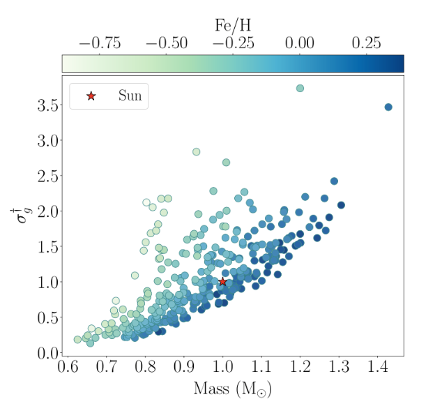
Using this mathematical model, they take a well-studied sample of stars with precisely known stellar parameters and compute the RV scatter from convective blueshift. Through this exercise, they determine that higher metallicity stars are more likely to have less RV scatter from convective blueshift, see Figure 2. The authors attribute this to the fact that higher metal contents make the star overall less transparent, so it becomes harder to see the rising hot gas that creates the blueshift in the first place.
The authors then use this data set to compare their computed values to the known, observed values. They show that their model (black) fits the observed data (red) better than a previous paper’s model (blue). This is really promising! Overall, they find the range of scatter from convective blueshift goes from ~5 cm/s for K dwarf stars (cooler than our sun) to ~80 cm/s for F dwarf stars (hotter than our sun). The authors go on to discuss the implications of this finding. If stars naturally have a background RV noise level of 5 to 80 cm/s, this means that any signals of Earth-like planets hiding in the data will be totally overpowered by the convective blueshift noise! This makes finding those Earth-like planets even more difficult than it already is. The authors state that we need to better understand how to model this noise out of our data. They also conclude by saying that they hope others will use their methods when compiling lists of stars to be targeting in future surveys because estimating the convective blueshift scatter beforehand, survey designers can choose carefully which stars have small scatter and are therefore worth spending the resources to observe.
Featured Image Credit: Fig 1 Dalal et al. 2023