Title: MAUVE: An Ultraviolet Astrophysics Probe Mission Concept
Authors: Mayura Balakrishnan, Rory Bowens, Fernando Cruz Aguirre, Kaeli Hughes, Rahul Jayaraman, Emily Kuhn, Emma Louden, Dana R. Louie, Keith McBride, Casey McGrath, Jacob Payne, Tyler Presser, Joshua S. Reding, Emily Rickman, Rachel Scrandis, Teresa Symons, Lindsey Wiser, Keith Jahoda, Tiffany Kataria, Alfred Nash, and Team X
First Author’s Institution: Department of Astronomy, The University of Michigan, Ann Arbor, MI, USA
Status: Published in Publications of the Astronomical Society of the Pacific, Volume 136, Number 10 [open access]
In today’s bite we are revisiting the theoretical mission MAUVE (Mission to Analyze the UltraViolet universE) designed during the inaugural NASA Astrophysics Mission Design School (AMDS) hosted at the Jet Propulsion Laboratory in 2023. In our last bite about MAUVE we covered MAUVE’s technical motivation (the need for a new UV space-based mission), science cases and their connection to the Astro2020 Decadal survey (making progress towards answering the field’s most pressing questions) and briefly outlined the proposed instrumentation–a low resolution imaging spectrograph named THISTLE. Today’s bite will focus on outlining specific science objectives for mission design, using one of MAUVE’s science objectives as an example.
When developing a mission, it’s best practice to let science drive the design of both the mission and its instrumentation. But in practice what does that look like in practice? The answer lies in a complex table called the Science Traceability Matrix (STM; Table 1 in today’s paper). The STM fundamentally outlines the most important details of the science objectives: which decadal goal(s) the science is linked to, what physical parameter must be measured to answer the science question, and what kind of observation is required to obtain the measurement. It’s easy to get physical parameters and observables confused, but it is important to understand the differences!
- Physical parameters describe something we are observing but cannot be directly detected (e.g. from MAUVE’s STM: ejection velocity of escaping atmospheres, energy release rate rise time for kilonova cooling mechanisms, or how quickly the surrounding material near a type 1a supernova is heated by shocks).
- Observables are directly measured or detected by instruments (e.g. from MAUVE’s STM: spectra and flux).
Answering the Science Objective
Once the physical parameters and observables are defined, it’s time to get specific about the bare minimum requirements to answer the science objective. It’s important to define the minimum information needed to answer the science question–since science in space is expensive! Designing for dream mission capabilities rather than what is strictly necessary to answer science questions can inflate mission cost to unreasonable levels very quickly. Let’s use MAUVE’s science objective O1 as an example:
- Science Objective: To determine whether sub-Neptune atmospheric escape is caused by photoevaporation or core-powered mass loss. (If you want some more background on why we care about how exoplanets lose their atmosphere, check out this Astrobite from Clarissa.)
- Physical Parameter: Ejection velocities between 0-20 km/s with a 1-2 km/s precision.
- Observables:
- Atmospheric transmission spectra of the Lyman-alpha line with transit depths up to 50% absorption with 1% resolution
- Stellar flux from the host star specifically between 50-91.2 nm.
Physical Parameters and their Precision
Ejection velocity probes how quickly the planet’s atmosphere escapes into space. Photoevaporation drives mass-loss rapidly with a 10-20 km/s ejection speed, but core-powered mass loss is much slower with an ejection speed of 1-2 km/s. So we know that in order to answer this science question we have to be able to observe ejection speeds between 0-20 km/s at minimum.
It is not just the ejection velocity range that matters, but also how precisely we need to measure the ejection velocity. This is especially important because we need to be certain that we will be able to distinguish between the two hypotheses the objective poses with our mission. If we build an instrument that can measure ejection velocities between 0-20 km/s but the precision on those measurements is +/- 10 km/s we won’t be able to answer the science objective since all of our ejection velocities will blend together within the error! A precision of 1-2 km/s will allow us to clearly separate photoevaporative atmospheric escape from escape driven by core-powered mass-loss processes.
Observables and Obtaining the Physical Parameter
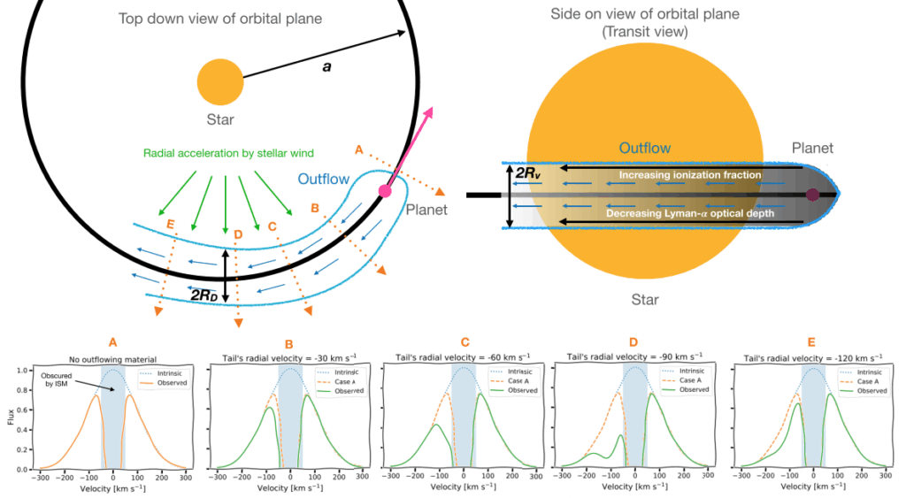
An atmospheric transmission spectrum is a spectrum of an exoplanet taken when the exoplanet crosses in front of its host star from our point of view (see the top right of Figure 1). Some of the light from the star that passes through the planetary atmosphere will be absorbed and some of it will be transmitted, leaving behind a spectral pattern that tells us the composition of the exoplanetary atmosphere (see a more detailed example of a model Earth-like exoplanetary transmission spectrum here). Lyman-alpha helps us monitor when excited hydrogen atoms (in this case, excited by stellar radiation) return to lower energy levels or de-excite, and the shape of the Lyman-alpha emission line (see the bottom row of Figure 1) tells us characteristics of the hydrogen tail outgassing from the planetary atmosphere.
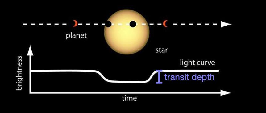
The transit depth specification for the atmospheric transmission spectrum observable is broken into two parts: the upper detection limit of specifically the Lyman-alpha transmission spectrum absorption level they hope to observe (this is the 50% absorption value) and the minimum transit depth precision they would like the instrument to reach (this is that 1% value). Figure 2 shows what we traditionally mean by “transit depth”: the amount of light obscured from the star while the planet passes between us and the star during an observation. The transit depth outlined for this requirement is slightly different–it refers to what percentage of the transit depth is specifically due to the absorption of hydrogen from the exoplanetary atmosphere–not the solid mass of the planet. So this requirement is indicating that the instrument needs to be sensitive enough to perceive absorption in the Lyman-alpha line flux at 1-1.5% of the transit depth–super precise!
We also want to know how much hydrogen ionizing stellar flux the planetary atmosphere is exposed to over time, so we can better model how the optical depth of the neutral hydrogen tail from the escaping planetary atmosphere changes with time. The stellar flux that ionizes the hydrogen in a planetary atmosphere mostly emits between 50-92 nm.
With both the Lyman-alpha absorption profile shape and the stellar ionization rate over time, we can determine the ejection velocity for several sub-neptune exoplanets These ejection velocities can help identify the primary cause of exoplanetary atmospheric loss, directly addressing the science objective posed!
Summary
Once again, MAUVE is not being developed further as a mission concept, but we can use papers like this one that outline mission design concepts in detail to piece together the best practices for crafting successful mission proposals! Science objectives are the foundation for a mission, so making sure they are well crafted, well connected to the decadal, and have clear physical parameters and observables with evidence based precision requirements is key. In today’s bite, we walked through only one of the science objectives for MAUVE, but there are 4 more objectives featured in the paper you can use to practice walking through the crafting and reasoning of science objectives! In our next installment in this mission design mini-series, we’ll discuss how science requirements inform instrumentation design requirements.
Astrobite edited by Niloofar Sharei.
Featured image credit: My cooked sense of humor and Pixlr Advanced Photo Editor.