Today’s coverage is focused on the DESI DR2 results, which have been published today in the Physical Review Journal (see the published papers on their Astro website, go.aps.org/astro). For more information about Astrobites’ partnership with APS, see this Astrobite.
This is Part 2 of our coverage of the DESI DR2 results. For Part 1, see this Astrobite, and for Part 3, see this Astrobite.
Paper title: Construction of the Damped Lyα Absorber Catalog for DESI DR2 Lyα BAO
Paper first author: A. Brodzeller, Lawrence Berkeley National Laboratory
Paper status: Published in PRJ [open access]
From Part 1 covering the DESI DR2 results, you might recall reading about how we can extract the BAO signal from the Lyman-alpha forest. To briefly recap this, as light travels towards us from distant quasars (galaxies with active galactic nuclei), there can be absorption of that light due to intervening neutral hydrogen at different redshifts along the line-of-sight, and that absorption is apparent as a series of lines in the quasar spectra – we call this the Lyman-alpha forest. That absorption traces out the matter distribution in the Universe, and thus can be used to probe the BAO signal – an excess clustering of galaxies (or in this case, absorption of light by neutral hydrogen) on scales corresponding to the sound speed at the time recombination occurred.
However, there is quite a bit of work involved in order for us to put together a catalog of quasar spectra that have the Lyman-alpha forest signal we are interested in. Sometimes, the density of hydrogen is so high that rather than just getting narrow absorption lines that we see in the Lyman-alpha forest, we get a line with broad ‘wings’ (see Figure 1).
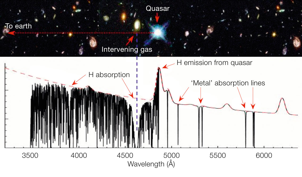
Figure 1: The spectrum from a quasar showing hydrogen absorption (the Lyman-alpha forest) and strong absorption profiles from dense intervening gas – i.e. damped Lyman-alpha absorbers (labelled by H absorption on the figure). Image credit: John Webb/ESO (CC BY 4.0)
We call these systems damped Lyman-alpha absorbers (or DLAs for short). While these systems can be used to trace much of the neutral hydrogen in the Universe, these systems are actually a contaminant for the standard BAO analysis of the Lyman-alpha forest, and need to be carefully identified to ensure they do not impact the BAO analysis. The shape of the line profile from these systems can introduce unwanted correlations and noise to the data products used to extract the BAO signal, so the DLA regions need to be “masked” (i.e., removed) from the spectra.
Here, we discuss the supporting paper that explains the work the DESI collaboration did to handle the DLAs. They produced the “DLA Toolkit”, a pipeline that identifies and masks the DLAs from the quasar spectra. In a nutshell, the DLA Toolkit models the intrinsic quasar spectra and separately injects a model for the features that enter the spectra when DLAs are present. This is then compared to a spectrum from data (or from mock data), and the best fitting model (either a spectrum that has no DLAs, or one DLA, or two DLAs, etc) is compared to find the best fitting model. For DESI DR1, two other existing tools in the literature were used together in order to find DLA contaminants in the data rather than this toolkit: a convolution neural network (CNN) trained on artificial DLA profiles injected into quasar spectra, and a gaussian process (GP) model that returns the probability of there being DLAs in the quasar spectra.
Testing the DLA Toolkit
Compared to DESI DR1, in which the DLA catalog is constructed using the existing CNN and GP methods, the DESI DR2 DLA catalog is constructed using all three of the DLA Toolkit, the CNN, and the GP method. Before applying these pipelines immediately to the data, they need to be tested on mock data to ensure they work correctly. In this work, realistic mocks for quasars in the DESI DR2 data are used, and DLAs are injected into the spectra to test the performance of the methods. True detections of DLAs in spectra are confirmed for each method by comparing the estimated redshift of the DLA (the redshift essentially tells you about where the DLA is relative to the quasar and the observer along the line-of-sight and is determined by the position of the feature in the quasar spectrum) and the column density (the density of gas along the line-of-sight) of the DLA to the true values input to the simulated spectra, and all three methods have their own parameter to quantify the significance of the detection. This has the benefit of obtaining a more complete list of DLAs in the data with more of the DLA detections corresponding to “true” DLAs (rather than false positives). Since each method has pros and cons, cross-checking results between the different methods allows for false positives to be removed and allows for some detections that are uniquely contributed from each of the methods.
The authors thoroughly test the impact of different thresholds for parameters used to determine the significance of a detection, DLA column density, and even the signal-to-noise of the quasar spectra for each method, to optimise the purity (fraction of true positives) and completeness (fraction of true detections out of all present in the mocks). They also test the impact of including broad absorption lines (BALs, from absorption by carbon, oxygen or nitrogen) in the spectra. These can be confused with DLAs by the algorithms. The CNN method does not rely on an intrinsic model of the quasar spectrum so is less susceptible to false positives caused by BALs in the spectra. However, it does have a tendency to underestimate the column density of the DLAs by a consistent offset, while the DLA Toolkit and GP method have increasingly accurate measurements of the column density with a higher threshold for the signal-to-noise of the quasar spectra. All three methods are able to predict the redshifts of the DLAs with equal precision. The catalog of DLAs compiled by detection from the three methods had 93.8% “true” DLAs (rather than false positives). This testing and work is essential to construct a reliable catalog of DLAs for masking the Lyman-alpha forest spectra used in the DESI DR2 BAO measurement.
The DLA catalogs and summary
For application to the real DESI data, the candidate DLAs must meet particular criteria for detection from at least the GP method with either the CNN or DLA Toolkit; the GP method is used as the common method, since it has the best accuracy for estimating the column density of the DLAs. For DESI DR2, the resulting catalog contains 41,152 DLA candidates out of 942,946 quasar sightlines; this was used to eliminate contaminating DLAs for the BAO analysis.
To estimate the purity of the real sample of quasars, they perform one more analysis. Essentially, true DLAs should have almost no flux transmission in the centre of the DLA absorption feature, particularly when most of the absorption is due to redshifted wavelengths that match any of the wavelengths of the Lyman series up to Lyman-10 (essentially, absorption of photons by hydrogen for any of the first 10 hydrogen energy levels). By stacking multiple spectra together (after they have all been shifted into the reference frame of the DLA), noise can be reduced relative to individual spectra to better study the DLA absorption for the Lyman series wavelengths. By doing so, they can see what fraction of the total flux (relative to a normalized flux continuum – that is, the continuous background flux that is intrinsic to the source) is transmitted at the centre of the DLA absorption feature for each of the first 10 Lyman series lines, and use this to estimate the fraction of contaminants in the DLA sample. Based on the flux transmitted through the Lyman-8 absorption feature (which they find to be sufficient in this work) they estimate the sample is about 76.3% pure.
The authors note that in future work, it may be possible to make improvements to the process of obtaining the DLA catalog from data, by improving some of the weaknesses identified in each of the three methods used in their work. Additionally, the quasar flux model they use in the DLA Toolkit has been trained on SDSS quasars, rather than DESI quasars. The modelling could be based on DESI quasars in future work to improve the DLA Toolkit. However, the work here has allowed for a DLA sample to be constructed with optimal purity and completeness. This work played an important role in allowing DESI to perform a highly sophisticated BAO analysis with the latest data.
Paper title: Validation of the DESI DR2 Measurements of Baryon Acoustic Oscillations from Galaxies and Quasars
Paper first author: U. Andrade, Leinweber Center for Theoretical Physics, University of Michigan
Paper status: Published in PRJ [open access]
So you have a one-of-a-kind dataset of 14 million galaxy and quasar spectra and you’d like to use it to make the most precise measurement ever of the most mysterious substance in the universe. How do you check your work? That’s the topic of validation, the subject of this paper.
Like many modern experiments, DESI blinds its data – meaning, the real values of the data are hidden from the astronomers working on the analysis – until the analysis pipeline is finalized. The idea is not to let what you expect the results to look like to affect the choices you make on how to handle the data. The analysis pipeline is first developed and tested using mock galaxy catalogs which come from giant cosmological simulations. Then, the pipeline is run on a blinded version of the data which has offsets applied to the redshifts of all the galaxies. After passing a series of checks, the pipeline is frozen and run on the real data, and at the end a set of pre-determined checks is made on the final result.
DESI has already conducted this process before with the first data release, and the DR1 pipeline is mostly kept in place for DR2. Some minor updates to the process are noted in the paper, mostly made to take advantage of the more sophisticated fitting and error estimation possibilities enabled by a larger amount of data.
What kind of checks is it possible to make? For one, you can do your math more than one way and see if you get the same result. The typical scales on which galaxies cluster can be quantified by more than one measure; by default, DESI uses the two-point correlation function in its calculations, but the authors also try using the spatial power spectrum to make sure it gives the same result.
Another big category of checks is splitting the data in various ways, calculating the BAO parameters separately on the different pieces, and seeing if the answers agree with each other. Why might this matter? Different galaxies are located in different parts of the sky, were chosen to be measured by DESI by different surveys, or have higher or lower magnitudes or stellar masses compared to others in their bin. The splits check whether effects from any of these non-cosmology-related factors are creeping into the results. There is also one redshift bin in which both the farthest luminous red galaxies and the closest emission line galaxies are present; the authors check whether the answers from the two galaxy types agree with each other in the overlapping range.
Finally, although DESI DR2 is the most precise BAO measurement to date, you can certainly compare to previous BAO measurements. The DR2 measurement is statistically consistent with both DESI DR1 and SDSS and has the lower level of statistical scatter you’d expect from the larger amount of data. DR1 and SDSS mildly disagreed with each other in one redshift bin, and the DR2 result for that redshift bin falls in the middle, supporting the idea that the earlier disagreement was a statistical fluctuation and nothing to worry about.
The DR2 results passed all the checks (many more than highlighted here!), increasing confidence in the conclusions of the key papers. The authors note that DESI’s overall uncertainty is still firmly dominated by statistical rather than systematic uncertainty: the systematic uncertainty is less than 6% of the statistical uncertainty. Nonetheless, as more data comes in and the measurement becomes more precise, modeling of systematic effects becomes increasingly important, and the authors plan to keep looking increasingly deeply at them in future work.
Paper title: Validation of the DESI DR2 Lyα BAO analysis using synthetic datasets
Paper first author: L. Casas, Institut de Física d’Altes Energies (IFAE), The Barcelona Institute of Science and Technology
Paper status: submitted to PRJ [open access on arXiv]
This paper discusses the validation process for making the BAO measurement from the Lyman-alpha forest measurements. Compared to DESI DR1 which had over 420,000 Lyman-alpha forest spectra, DR2 has more than 820,000 Lyman-alpha forest spectra. An important part of the analysis is to apply the measurement pipeline to mock data (simulated data). This ensures that we are aware of how accurate and precise our measurements are when applied to the real data, and to quantify any uncertainty in the measurement; this is especially important to ensure the validity of our scientific claims discussed in the other bites. This paper discusses the process to make the 400 mocks for the DR2 data (compared to 150 for DESI DR1) and apply the measurement pipeline to these mocks for computing the BAO parameters – specifically for Lyman-alpha forest measurements. It also discusses the improvements made to the mocks for this compared to DR1 and measurement pipeline for DR2.
Mock creation process
In a nutshell, the mock creation process starts with initiating a matter distribution that can be described by a gaussian random field. The matter field then needs to be populated with quasars, and a biasing model (see here for more information on galaxy bias) is used to ensure the density of quasars follows an expected distribution that depends on the matter density; essentially, galaxies or quasars are not perfect tracers of the matter field in the Universe, and may be more likely to be found at regions with a critical density of matter. This is an important effect that needs to be included to accurately simulate the correlations between quasars for the real BAO measurement. After this, the density of matter along the line-of-sight to the quasars can be used to estimate the flux that is absorbed from the spectra of quasars by the Lyman-alpha forest.
Since the measurements of the BAO from DESI DR1 with real data had more uncertainty than was found from the measurements with mocks, the authors have included more impacts of non-linear evolution in the mock data for the DR2 measurement. Neglecting this effect in the modelling of the quasar correlations could lead to a less precise BAO measurement, so they account for this in DR2. By comparing the DR2 mocks to highly accurate (but computationally expensive) N-body simulations, they find these mocks do have more accurate uncertainty properties.
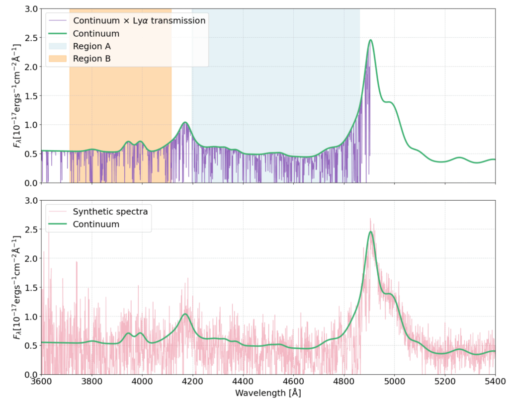
Finally, they need to make sure the mocks are a representative sample of the real DR2 data. As such, they ensure the mocks match the ‘footprint’ (basically the map of galaxies across the sky) and redshift coverage for quasars from the DR2 data, and similarly for the magnitude (essentially the measured brightness) of each galaxy. The quasar spectra in the mock data also need to have noise (essentially some randomness in the flux) that matches that seen in the real data for it to be realistic – you can see this in Figure 2 below, which shows an example mock spectrum. They finally include the impact of redshift errors in the mocks, since errors in the estimated redshifts can contaminate the measured correlations between quasar spectra. Including them in the mocks can give the authors a better idea about how well we can truly measure the quasar correlations.
Measuring the correlation function
To validate the mocks are representative of the DESI DR2 data and apply the BAO pipeline, they calculate correlation functions for the fluctuations in the Lyman-alpha forest in two distinct spectral regions (see the shaded regions in Figure 2) and also the correlations of these fluctuations with the quasar position themselves; this leads to six distinct correlation functions. The correlations tell us about the excess chance of seeing Lyman-alpha forest absorption (or the presence of quasars) separated on different length scales, and we expect to see a bump or dip corresponding to the BAO feature (or essentially the scale that corresponds to the when the sound waves that travelled in the early Universe froze in place, discussed more in Part 1 – this is essentially our ‘BAO ruler’). This feature is similarly seen in the correlations of other galaxies. For the quasar analysis, this correlation function is computed separately for separations between quasar positions or Lyman-alpha forest fluctuations a) along the line-of-sight and b) perpendicular to the line-of-sight. By computing the correlation functions from the mock data and comparing that to the real data, the authors can see the mocks are a good representation of the real data.
In order to obtain the BAO parameters of interest (essentially the thing that gives us our calibrated ‘BAO ruler’ and informs us on the expansion rate in the past), we need to fit a model to each of the six correlation functions. The model used for the correlations between the Lyman-alpha forest fluctuations and quasar positions can be computed using a cosmological model (that essentially can give the correlation function for the underlying matter field). Then it takes into account impacts like motions of the matter field due to gravitational interactions (called peculiar velocities), biasing in the quasars and forest fluctuations relative to the underlying matter distribution (the biasing model), the finite binning of the data, small non-linear corrections (related to non-linear evolution mentioned earlier) and unwanted correlations with metal absorption lines. Additionally, the algorithm discussed earlier for masking DLAs is applied before measuring the correlation function. After the model fitting, the ‘BAO ruler’ can be extracted from the mocks (and also the real data later).
Validation of the BAO analysis
Finally, we can get to the main and most important test, which is to check the BAO parameters we extract from the data are robust to different modelling choices, and obtain some idea of how accurate our analysis pipeline is based on the mock data. The authors perform a fit to a correlation function obtained by combining the measurements from all the mocks (this gives a measurement with very high signal-to-noise) and also fit the individual mocks. From the combined fit, they do find a small – but significant – bias in the measured BAO parameters compared to what they expect to find based on the ‘truth’ of the mocks. They are able to determine that this bias is largely due to the impact of including errors in the measured redshifts of the absorption lines in the quasar spectra, which was included to make the mocks more realistic representations of the real data. By removing this impact and reanalysing the mock data, the results are more accurate. This confirms this is in fact the source of bias in their tests, and it could impact the measurements of the real data. How can they deal with this for the real data, where redshift errors cannot necessarily be avoided?
The authors make one modification to their analysis, which is to remove measurements of correlations that come from pairs of quasars that are closer together. They base this choice from results of previous literature, which show that this choice largely mitigates the impact of redshift errors in the results, and they find this works well with the mock data in their own tests. Overall, the final result is that they obtain measurements with the mock data that satisfy the requirements they demand for the analysis on the real data regarding accuracy and precision. Overall, they demonstrate the pipeline for the BAO analysis on the Lyman-alpha forest is sufficiently reliable; you can trust the authors have thoroughly tested the analysis that leads to the fascinating results discussed in Part 1.
To read more of our coverage of the DESI DR2 Results, return Part 1 or check out Part 3!
Edited by: Brandon Pries and Jessie Thwaites
Featured Image Credit: DESI Collaboration/KPNO/NOIRLab/NSF/AURA/P. Horálek/R. Proctor (CC BY 4.0)