- Title: Fundamental Stellar Parameters and Metallicities from Bayesian Spectroscopy: Application to Low- and High-Resolution Spectra
- Authors: Ralph Schönrich and Maria Bergemann
- First Author’s Institution: The Ohio State University, USA and University of Oxford, United Kingdom
- Paper Status: Submitted to MNRAS
The link between a pile of data and a physical explanation is the fun part. Astronomers spend countless hours gathering data, and countless more thinking up physical models for different pieces of the Universe. But reconciling these two things—finding a model that not only agrees with observations, but is the sole likely explanation—isn’t easy.
Consider the spectrum of a star. Depending on the star’s temperature, surface gravity, and chemical composition—also known as metallicity—a spectrum can look different in subtle ways. To characterize a star based on its spectrum, a common technique is to create many theoretical model spectra. Then, you use another tool to decide which model spectrum best matches your observed spectrum. Once you pick one, that model’s values for temperature, surface gravity, and metallicity are used for the star you observed.
In a general sense, this is straightforward. But in reality, it can get messy quickly. What if there are more than three properties I need to model? What if I observed the star more than once? What if I use two different programs to create model spectra and they don’t agree? What if my observed spectra are noisy, or from different telescopes and instruments? What if more than one model matches equally well with my observation? And how do I decide which model “best matches” my observation, anyway?
A new way to derive physical parameters from spectra
In this paper, Schönrich and Bergemann present a whole new suite of tools to address this common task. Instead of fitting one model to one spectrum, with custom answers to all of the previous questions on a case-by-case basis, they take a step back and whip out some Bayesian statistics. Instead of asking, “Which model fits the data best?” they ask, “Given a set of observations, what combination of physical parameters is most probable to exist?”
To answer this question, they show how to calculate a Bayesian probability distribution function (PDF) for many parameters at a time. Think of each parameter as an axis on a graph: for two parameters, like temperature and surface gravity, the PDF could be plotted on a piece of paper. For three parameters, you would need a 3D graph. The same math lets you consider an arbitrarily large number of parameters at once, even if you can’t visualize a graph of it. And for each source of data that constrains the problem (an observed spectrum, or even photometry), a new multi-dimensional PDF can be generated. These PDFs can then be combined to yield an overall most-likely solution.
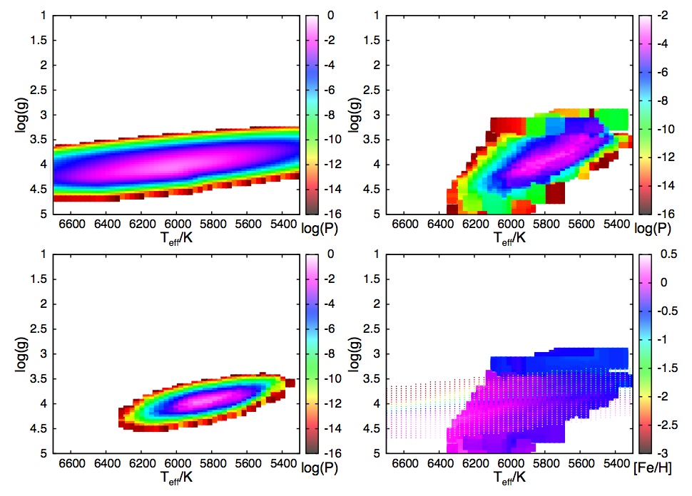
Probability density functions (PDFs) for one star. In three of four panels, probability (log(P)) is shown in color in the surface gravity (log(g)) vs. temperature (T) plane. Top left: PDF based on photometry and a stellar evolution model. Top right: PDF based on spectroscopy. Bottom left: combination to make the overall PDF. Bottom right: expected metallicity from the photometry + stellar evolution model PDF (dots), and from the spectroscopy PDF (colored area). The most likely solution is the one with log(P) closest to 0 (probability closest to 1).
Bayes on trial
This sounds great in theory, but how is it in practice? To test this, Schönrich and Bergemann apply their method to both high- and low-resolution spectra from different instruments. For two samples of stars, they look at how the derived temperatures T, surface gravities log(g), and metallicities [Fe/H] line up with physically realistic expectations. Both samples of stars were previously analyzed using a more conventional method. They find that the new Bayesian technique consistently does a better job, because it doesn’t have any stars in so-called “unphysical” locations in the T-log(g)-[Fe/H] parameter space. In both cases, the stars better populate the Main Sequence with the new method, and they more consistently follow lines of constant age (called isochrones).
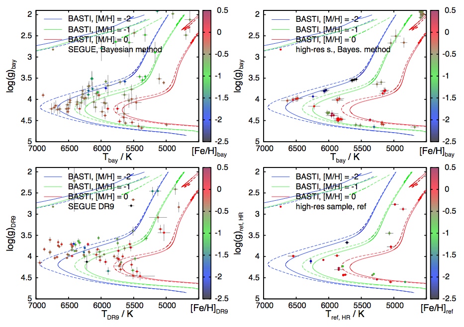
A comparison of the Bayesian method vs. traditional modeling for two samples of stars. (Dots on each plot represent stars, while the lines are isochrones for reference). The low-resolution spectra are on the left, and the high-resolution sample is on the right. The new technique is shown in the top panes. For both samples, stars in unphysical positions—not roughly consistent with the isochrones—disappear with the Bayesian method, whereas they are present in both reference samples.
A widely-applicable, robust technique
The tools presented in this paper are useful for many situations, from simple cases like the opening example—understanding a single star—to analyzing huge datasets from surveys in a consistent manner. The authors even suggest that the same Bayesian framework could be used to include other datasets that constrain physical quantities: astrometry, interferometry, and asteroseismology, to name a few.
Beyond being widely-applicable, the authors emphasize that their method has advantages over other available approaches. It can consider all observational and theoretical data available for a star, it is robust with respect to low-quality or missing data, it handles uncertainties well by considering the full multi-dimensional PDF, and it is well-suited for comparing data from different surveys to one another.
Author
Trackbacks/Pingbacks