This post is written by Benjamin Nelson, a graduate student in the Astronomy Department at the University of Florida. He works with Dr. Eric Ford on the characterization and dynamical evolution of extrasolar planets. He is currently developing an N-body Markov chain Monte Carlo for RV observations of exoplanet systems.

Why is this important to astronomy?

Inevitably in your astronomical career, you’ll attend some talk where the speaker mentions “MCMC” and “Metropolis-Hastings”, or maybe something about “priors” and “likelihood functions.” The latter terms refer back to a Bayesian framework, while the former terms are the numerical tools, both of which are rarely covered in undergraduate astronomy/physics. Although Bayes’ theorem has been around for more than 200 years, computational advances within only the past couple decades have made it actually practical to solve problems involving Bayesian techniques.

Learning statistical methods is like eating your vegetables: you probably won’t enjoy it, but it’ll be good for you in the long run. It is hardly motivating for an astronomy grad student to pick up an introductory book on Bayesian statistics without some practical application in mind, but a solid knowledge of Bayesian methods is a great way to find common ground in other, unfamiliar astronomical subfields, or even other disciplines of science. The purpose of this astrobite is to familiarize the reader with conventional Bayesian jargon (sugar coated with some astronomy) and lay out the ingredients to code a Markov chain Monte Carlo from scratch.

Bayes’ Theorem:

In short, Bayes’ theorem allows us to update our knowledge of a model system using new sets of observations. We use this to quantify the uncertainties of the underlying set of model parameters when we do not necessarily know the shape or scale of their respective distributions. For context, we will consider observations of extrasolar planets, a field I am particularly active in, but these methods work just as well for any astronomical specialization.

Figure 1: A synthetic RV curve of a 1-planet system (100 days, 1 Jupiter mass, 0.5 eccentricity). How do the errors, , in the RV observations, , translate to the errors in period/mass/eccentricity/etc.?

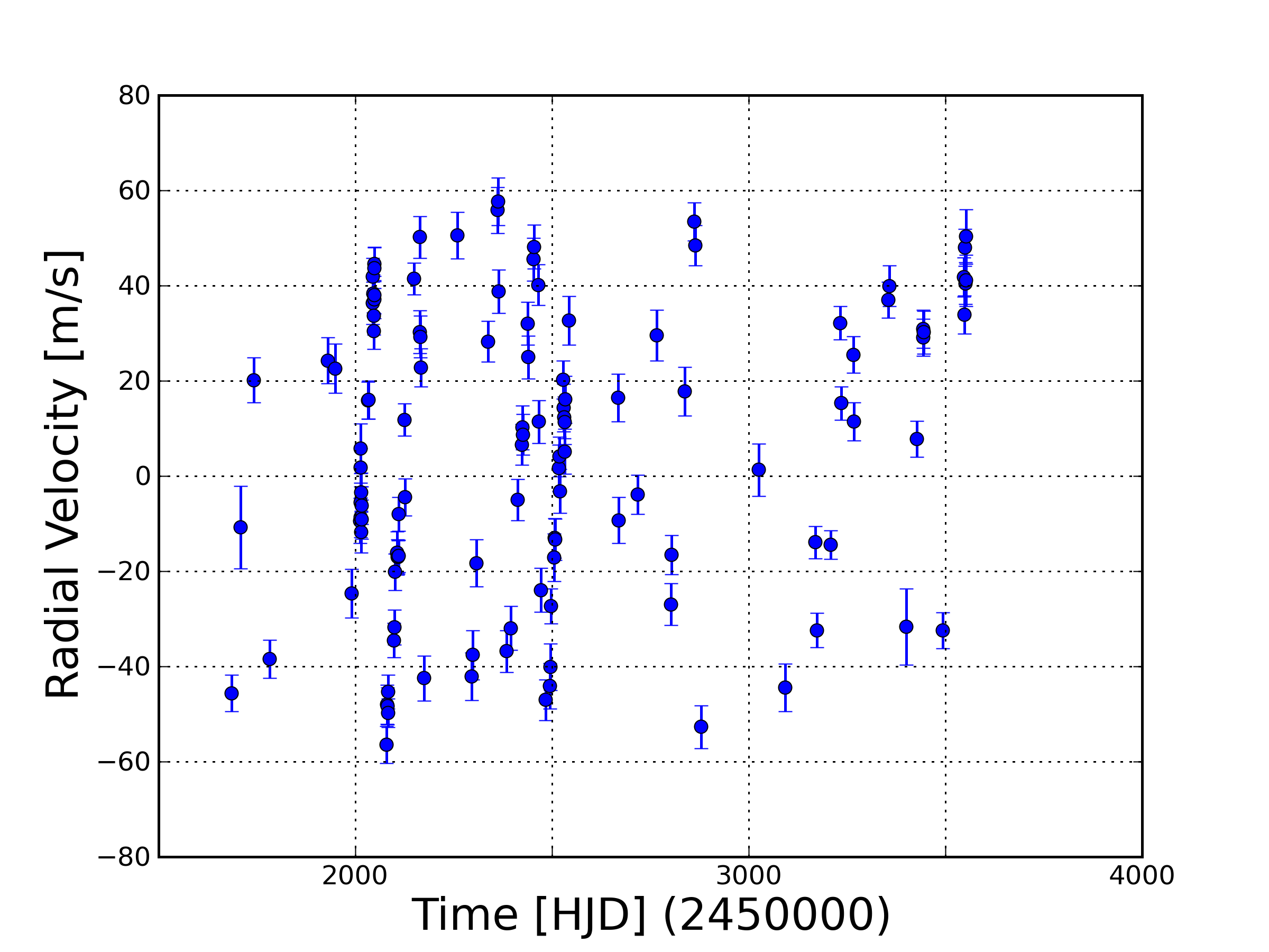
Let us consider a radial velocity (RV) curve of some star (Figure 1). Refer to this astrobite for more on the observational method. These RV observations have some random measurement uncertainty and some extra error due to systematics and astrophysical noise sources. The latter is often lumped into a term called “jitter“, . We want to pin down the orbital properties of the planetary system that best models these observations and their associated uncertainties. However, we have 7 model parameters for each planet: three positional components, three velocity components, and mass. Thus, a simplistic 2-planet model already requires us to explore a 14-dimensional parameter space, excluding jitter and RV offsets from various instruments. With such a seemingly daunting task at hand, how do we possibly estimate the uncertainty in our set of model parameters? This is what we are ultimately after.

Let’s begin with the actual definition for Bayes’ theorem:

The “posterior” probability distribution, , is proportional to the product of the “prior” probability distribution, , and the “likelihood” function, , all defined below. is a normalizing factor called evidence, which isn’t necessary to compute for the computational methods soon to be discussed.

Likelihood:

The formal definition of the likelihood is the probability of obtaining a set of N observations, , given a known model and its set of model parameters, . In the exoplanet context, let’s assume that each of our RV observations, , were made independently. We’ll also assume the errors in the RVs, , have a known magnitude and are normally distributed and uncorrelated. We can construct the appropriate likelihood function,

is the theoretical model that fits the dataset, so our likelihood is a function of our model parameters. The specific shape of the likelihood function is still difficult to visualize, especially if is a complicated, non-analytic model.

Prior:

A prior is something that summarizes something about a particular parameter before we make any new observations. When adopting a prior, there are two general flavors: broad and informative.

Say we observe an evolved F sub-giant. Based on this knowledge alone and no RV data, could we hypothesize what kinds of planets orbit this star, specifically their orbital periods, eccentricities, etc.? There might exist some weak correlation, but until we know this, it’s safer to make no assumptions. So, we set up some broad priors. For instance, we could set eccentricity and phase angles to be uniform over their respective domains. For a parameter with no upper bound like orbital period, we could adopt something like
. The intent here is that the likelihood is so sharply peaked that it dominates the shape of the posterior rather than the prior.

Is there any model parameter that we could constrain based on the type of star in question? Maybe, we can consider the jitter term, , mentioned before. Going through the literature, we find this type of star has a median jitter of 5.7 m/s with ~1-sigma confidence intervals at 4.6 and 9.5 m/s (Wright 2005). With this, we could create a distribution of similar properties as our prior. This informative prior specifies that such a star would not be responsible for relatively large jitters.

Posterior:

The product of the likelihood and prior distributions gives us the posterior, our desired distribution. Easy enough. Now, we want to quantify the uncertainty in our model parameters using this multidimensional posterior distribution, possibly arising from a horrendous looking likelihood and/or prior(s). A common solution nowadays is to utilize some numerical techniques that draw samples from the posterior so we can characterize the shape of the distribution. This is where Markov chain Monte Carlo comes in.

Markov chain Monte Carlo (MCMC):

The most common implementation of MCMC is a random-walk algorithm that estimates the posterior distribution so we can finally get some terms on our model parameters. In essence, we take a single model, a “state”, and perturb all of the parameters a bit, then determine whether this new model is better or worse. Through this acceptance process, we build a “chain” of states that can be used to create parameter distributions. The typical procedure is as follows:

1) We begin by identifying an acceptable model solution as a starting point. From here, we gauge how the well each of our model parameters is constrained and use this information to assign a list of “steppers,” the scale length to perturb each parameter value. Of course, being a Monte Carlo algorithm, there is a bit of randomness to the step, usually drawn from a random-walk proposal distribution. The good news is that the choice of steppers don’t have to be terribly accurate. An order of magnitude estimate is normally sufficient to achieve rapid mixing. A poor choice is steppers will lead to a very time-consuming exploration of parameter space.

2) From here, we calculate the posterior probability of this state,

3) Next, we apply a random step to our current state, and calculate the posterior probability for this new trial state

4) We compare the two posteriors. If is better than , we accept it as the new state. If it is worse, there is a chance it’ll still get accepted based on the ratio of their posterior probabilities. Note that because we are taking this ratio for the same physical model, it isn’t necessary to compute the evidence term, .

5) Go back to Step 3. Keep repeating until a “chain” of states is assembled. Sampling the chain will result in an approximation of the posterior distribution.

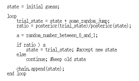
Figure 2 demonstrates the above procedure in a more algorithmic format.

Figure 2: The heart of any MCMC algorithm. Inspired by Skowron 2011.

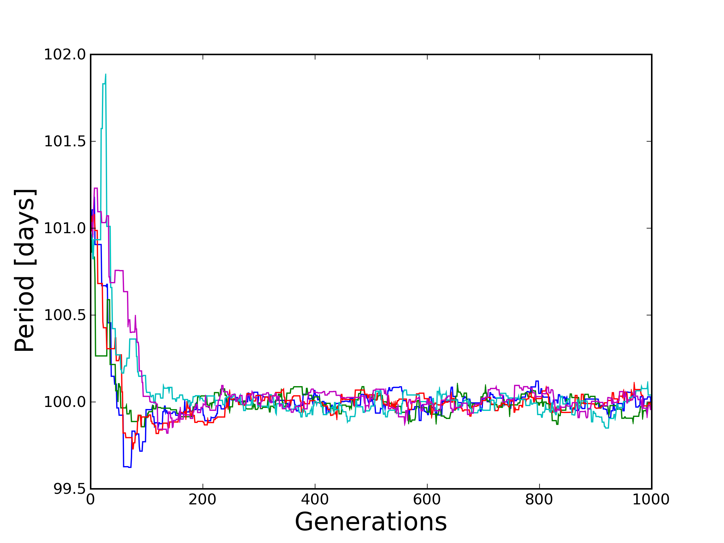
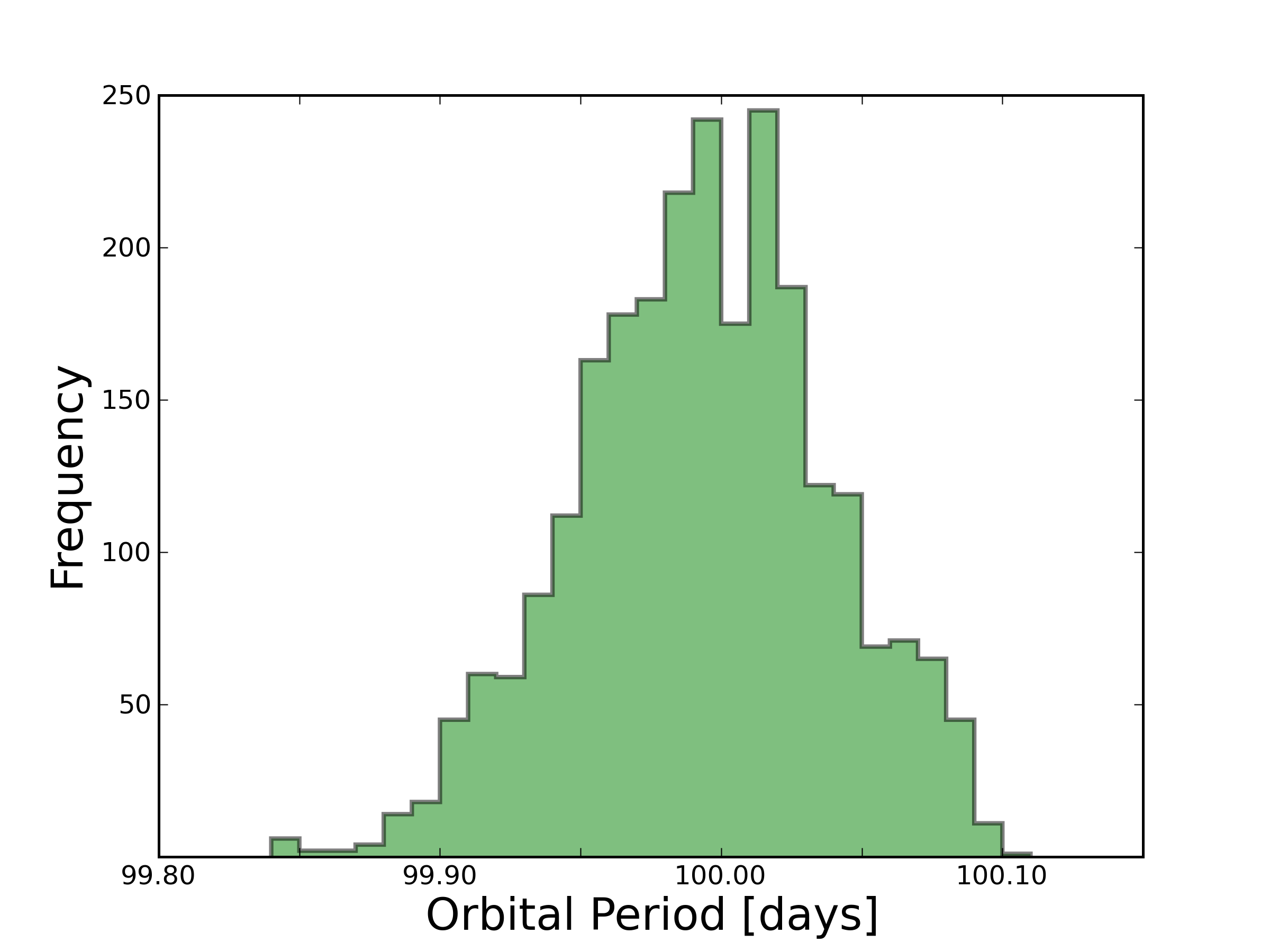
We now have the necessary components to code up a basic MCMC! Some further suggestions need to be addressed in order to make effective use of this computational tool. In a world of GPUs and parallel computing, it is most efficient to run multiple, independent chains and sample from all of them. It also provides us with a sanity check for convergence, since chains often get stuck in local minima. Depending on the initial guess, a Markov chain may wander and sample from these regions of parameter space before finding the mode of the global minimum. To obtain results insensitive to the initial guess, we throw out these states and, for safe measure, some of the generations of states that follow. This is known as the burn-in phase. Figure 3 shows the evolution of 5 Markov chains, from burn-in to convergence. Figure 4 forms a histogram of the converged states from Figure 3.

Figure 3: The estimated orbital period as a function of generation for my synthetic RV curve. Each color represents one of 5 Markov chains. I intentionally started them a bit off from the true orbital period to demonstrate the importance of the burn-in phase. Everything before the 200th generation looks like junk, but in order to avoid possible correlations with the initial guess, it’s best to throw out the next couple hundred generations as well.

Figure 4: A histogram of the last 500 generations of the MCMC in Figure 3. In order to characterize the distribution better, we would need to run the algorithm longer or run more Markov chains in parallel.

Finally, what does this “Markov” term mean? To be Markov, your next step only depends on where you are now, not where you have been (SMBC recently addressed a Markov thought process). This is important because a Markov chain should be able to explore all of parameter space without any historical bias influencing the shape of the sampled posterior. People often come up with clever schemes to make MCMC codes converge faster at the cost of being “pseudo-Markov” (referring to information from the chain’s history). If you wish to go down this route, prepare to justify your methods or feel the wrath of the Bayesian purists.

In summary, the methods described above allow us to take a model system and update the constraints on the model parameters based on new observations. This is especially helpful when simple error propagation formulas become tedious to calculate. There are certainly more complex issues worth investigating (how to deal with parameter correlations, parameter transformations, penalties). For further reading that panders to the physical sciences, I’d recommend this textbook.

—
Ford 2006, ApJ, 642, 505
Gregory 2005, Bayesian Logical Data Analysis for the Physical Sciences, Cambridge University Press
Skowron 2011, http://nexsci.caltech.edu/workshop/2011/talks/jskowron-mcmc.pdf
Wright 2005, PASP, 117, 657