Paper: Probabilistic Mass-Radius Relationship for Sub-Neptune-Sized Planets
Authors: Angie Wolfgang, Leslie A. Rogers, Eric B. Ford
First author’s institution: UC Santa Cruz
Status: Submitted to ApJ
Thousands of transiting exoplanets have been discovered, but for most of these planets we only know their radius and nothing about their mass. With a mass-radius relation, we can infer the masses of all these planets. This paper provides a new, probabilistic mass-radius relation for small planets, and its approach is somewhat unusual…
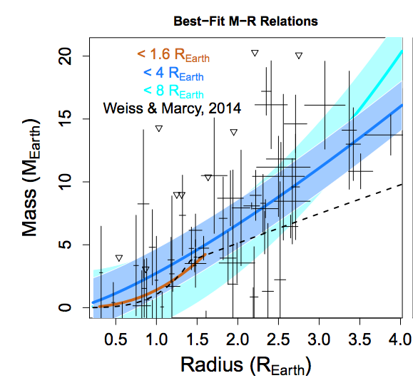
Figure 1. The mass-radius relation for sub-Neptune sized exoplanets. The exoplanets with both mass and radius measurements are shown in black. The resulting mass-radius relation is the solid blue line, and shaded blue region shows the intrinsic width of the line. This is figure 4 in the original paper.
Astrophysical dispersion in the Mass-Radius relation
A few dozens of exoplanets have both a radius measurement, because they transit their host star, and a mass measurement, because they cause enough reflex motion of their host star that we can measure their mass via the radial velocity method. All of the ‘sub-Neptune-sized’ exoplanets (those smaller than 4 times the size of Earth) with both mass and radius measurements are plotted in figure 1.
These data can be used to determine the mass-radius relationship for all small exoplanets, a super-useful thing to know because the majority of detected exoplanets only have radius measurements. With a nicely calibrated mass-radius relationship, we can predict an exoplanet’s mass, given its radius. But here’s the rub: the mass and radius measurements for these exoplanets don’t just fall neatly on an infinitely narrow line, there is a lot of scatter. Some of that scatter is produced by the noisy data, i.e. not every measurement is infinitely precise, so one would naively expect the measurements to fall slightly away from the best-fit line (68% of the measurements should fall within 1 \(\sigma\) of the line if the observational uncertainties are perfectly Gaussian). But the real question is, even if you knew the mass and radius of each exoplanet with infinite precision, like you could actually go to the planet with a tape measure and a set of scales and measure those things, would the masses and radii fall on an infinitely narrow relationship then? Wolfgang and authors show that the answer is no, and they quantify exactly how much intrinsic scatter there is in the relation between exoplanet mass and radius.
Hierarchical Bayesian Modelling
Hierarchical Bayesian Models (HBMs) are useful when you have layers of parameter dependencies. There are a few different sets of parameters in this particular problem. There are the parameters for the mass-radius relation, which is a power law, and there are the parameters that describe the distribution of masses that are allowed for a given radius. Wolfgang et al. assume a Gaussian distribution is a good description for this, and that Gaussian has a mean (the exact mass predicted for a given radius as computed using the mass-radius relation) and some standard deviation, \(\sigma\). Actually, this \(\sigma\) is a function of radius too: there is a smaller mass dispersion for small planets than for big planets.
So that’s the story. A set of parameters to describe the mass-radius relation and a set of parameters to describe the scatter in the mass radius relation. In a classical “fitting a model to data” situation, there is no extra set of parameters to describe the dispersion and relationships are just assumed to be deterministic (i.e., for a given radius there is one ‘true’ mass). Having these two sets of parameters is what makes this approach hierarchical. What makes it Bayesian is the fact that the authors use prior Probability Distribution Functions (PDFs), (they have beliefs about what the parameter values should probably be), and they explore the posterior PDFs of those parameters (the probability of the parameters, given the data). I won’t go into detail about Bayesian statistics here, take a look at this astrobite for more info.
Wolfgang et al. use Gibbs sampling to explore the posterior PDFs of the parameters. Their new model is shown in figure 1. The solid blue line shows the ‘best fit’ mass-radius relation and the shaded blue region shows the dispersion of this relation, \(\sigma\). The previous mass-radius relation from 2014 is shown as the dashed black line.
The point of it all
Say you know an exoplanet’s radius and you want to infer its mass. This model won’t just give you a ‘point estimate’ as an answer, e.g. “this planet should weigh exactly 3.215 times the mass of Earth”, it will provide you with a probability distribution over masses. This is a much more intuitive and informative way to think about measurements and inferences of parameters because almost nothing can be known with infinite precision; everything can be thought of as a probability distribution.
This paper is an important piece in an ongoing conversation about how we should treat relationships between parameters in general; most relationships are not deterministic! The methods used here should be more widely adopted, and are what makes this work such an essential component of the astrophysical literature!
Author