This guest post was written by Paul Rogozenski, a PhD student at the University of Arizona. Paul studies cosmology, researching the characterization of tension within cosmological sky surveys and extensions to the standard cosmological model.
Title: Reconstructing Probability Distributions with Gaussian Processes
Authors: T. McClintok, E. Rozo
First Author’s Institutions: Brookhaven National Laboratory, Upton, NY; University of Arizona, Tucson, AZ.
Status: Accepted to Monthly Notices of the Royal Astronomical Society [open access on arXiv]
Today’s astrobite takes a detour from typical observational astronomy to talk about the statistics of large sky surveys. Surveys often go through a grueling phase of theory before observations begin, where Monte Carlo Markov Chains (MCMCs) are usually used to infer model parameters from predictive data. The MCMC does not actually simulate data, but uses Bayesian statistics and what is known a priori about a physical model of interest (e.g. the standard cosmological model) to find best-fit values and their errors from inputted data. This is done by ‘sampling’ the probability distribution, or evaluating a probability distribution at a certain point in your model. The next sample is found by proposing a small change to the current sample, evaluating the probability distribution at the proposed point, and observing whether the proposed point’s values are more probable within the given model. Methods to effectively sample a probability distribution is an active topic of research and many frameworks exist to run MCMCs for cosmological surveys, like Polychord and CosmoMC.
Combining survey data is an excellent way to find better constraints on a model. Using MCMCs on independent surveys is computationally expensive, and using them on a joint survey is even more expensive. Separate surveys often measure separate model parameters, making comparisons between surveys and joint-data analyses difficult without running a computationally costly joint MCMC. The authors of today’s paper offer a simple method to infer joint distributions using MCMC runs from independent surveys.
What are Gaussian Processes?
The method, popular in machine learning, uses ‘Gaussian Processes’ to infer the probability values of points not directly sampled in an MCMC. Say there are some points in the data whose probability values are of interest. Calculating how these points vary with one another is the first step to inferring their probabilities. One of the underlying assumptions in Gaussian Processes is that the covariance between two points relies only on the two points considered (which is found by using a kernel). This makes finding the covariance matrices pretty simple, since the whole ensemble of samples need not be considered.Training data with known probability values are then carefully selected from the distribution. The training data anchors the inferred distribution to known values and is chosen to be evenly dispersed throughout the initial data (the authors use a Latin Hypercube to do this). It’s also necessary to determine how the training data covariance and how the training data varies with the points of interest. Now all there is left to do is to infer the probabilities at the points of interest using some matrix calculations (Equation 1 of the paper).
Great, but are Gaussian Processes accurate?
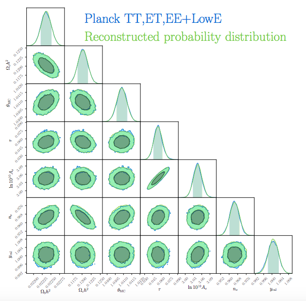
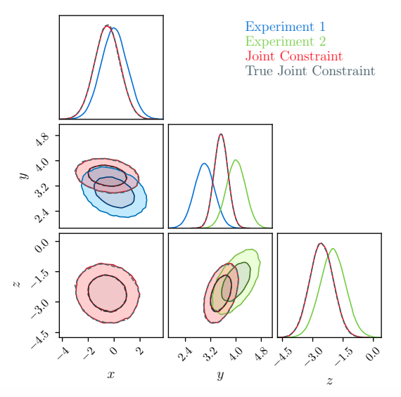
McClintok and Rozo use Gaussian Processes in a toy model to determine how well their methodology works. As seen in Figure 1, they take two normal distributions that have one joint parameter and see how well they can infer the true (analytical) solution. As you can see, they are spot on. The authors go further and infer real data from the Planck survey to see how their methodology scales to a higher-dimensional problem. Taking an MCMC run from the Planck 2018 results, the authors are able to very accurately recover the probability distributions of important cosmological parameters (Figure 2). The authors also note that their reconstruction took only about 30 minutes and retrieved 40 times as many samples as the original MCMC. In contrast, the Dark Energy Survey (DES) joint analysis with Planck took over 3000 CPU hours to compute: an incredible speed-up. Additionally, the error analysis of their reconstructed chains show a difference no more than about 0.2% from expected values (Figure 4 of the paper).
In summary, this paper outlines the method of inferring the probabilities of data points from known values with amazing speed and accuracy. This method of inference further raises important questions regarding computational expense. For instance, since Gaussian Processes recover probability distributions remarkably well, how long should one run an (expensive) MCMC before using (cheap) Gaussian Processes to infer more values? Are Gaussian Processes well-behaved in other surveys or in joint analyses? It is still an open question whether the method of Gaussian Processes will work well when joining two high-dimensional surveys (e.g. DES and Planck), which the authors defer to future work.