Authors: Jie Yu, Timothy R. Bedding, Dennis Stello, Daniel Huber, Douglas L. Compton, Laurents Gizon, Saskia Hekker
First author’s institute: Sydney Institute for Astronomy (SIfA), School of Physics, University of Sydney, NSW 2006, Australia
Status: Accepted for publication in MNRAS [open access on arXiv]
Long Period Variables
You usually can’t tell by looking with the naked eye, but the brightness of almost all stars varies with time. The study of oscillations in stellar brightness is called asteroseismology, and is one of the best methods we have to study the physics of different stars. If a star is exhibiting variability, it is usually due to things happening inside the star. The study of visible oscillations provides a window into a star’s internal processes.
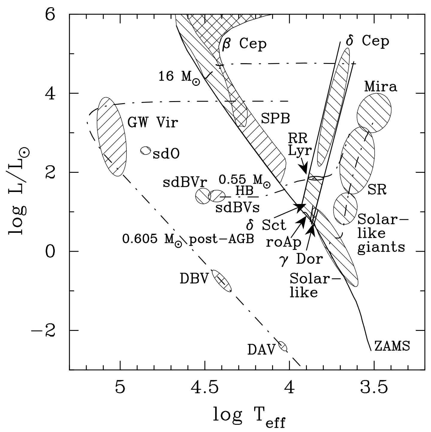
Figure 1: A Hertzprung-Russel diagram showing different types of variable stars. Of importance for today’s Astrobite are Solar-like oscillators & Solar-like giants, which oscillate in the same way as the Sun, and SR (semiregular variables) & Mira variables, which are classed as so-called Long Period Variables (LPV). This region of the HR diagram contains both Red Giant Branch stars and Asymptotic Branch Stars, which are both capable of being Long Period Variables. Circles hatched bottom-left to top-right exhibit acoustic waves, and vice-versa for gravity waves. For more details, see Handler et al. (2009, 2013). [Figure 1 in Handler et al. (2013)]
Today’s authors were interested in asteroseismology of so-called Long Period Variables (LPVs). This class of stars includes low-temperature, evolved stars on the Asymptotic Giant Branch (stars burning helium in shells around their cores) and on the tip of the Red Giant Branch (burning hydrogen shells). These stars, which experience brightness variability with periods of longer than a few tens of days, can be classified into Semiregular Variables (SRs) and Mira variables (see Figure 1).
Using a sample of 3213 LPVs observed with the Kepler space telescope and the OGLE survey, today’s authors aimed to have a look at a number of outstanding questions about these stars:
- Are their oscillations excited in the same way as solar-like oscillators, or as Mira variables?
- What overtones of the fundamental oscillations are we observing in these stars?
- And: if LPVs are like solar-like oscillators, can we apply the same techniques used to study those shorter-period variables?
Overtones of Oscillation
To understand today’s paper’s results, we need to first understand a little about how we describe modes of oscillation in stars. Much like in a string, we can describe different overtones of a standing wave using the number n. A mode of n = 1 is a fundamental oscillation, where all the material on a string moves up and down. The first harmonic, n = 2, has one node, where no material moves, in the middle of the string, and so forth.
In stars, where the standing waves propagate in a 3D space, n is referred to as the radial order, and describes how many shells of oscillating material there are, separated by unmoving nodes. For smaller stars like the Sun, we typically observe high-overtone modes (n ~ 20) on the surface. As we observe larger and larger stars, we observe lower overtones.
Finally, since a star is oscillating in 3D space, there are different shapes of oscillation, described by l, the angular degree. The three oscillations we can typically observe on distant stars are radial oscillations (l = 0), where the star inflates and deflates; dipole oscillations (l = 1), with a node along the equator; and quadrupole oscillations (l = 2), with two nodes wrapping around the star. Each of these oscillation types will have slightly different frequencies at each overtone, making them visible in long-time series observations.
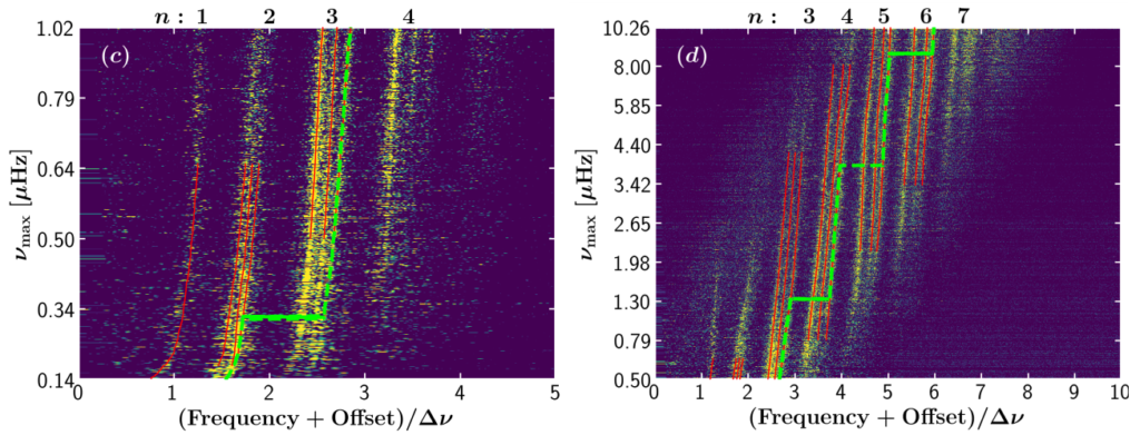
Figure 2: An echelle diagram of the observed SR variables. The y-axis, νmax, is the frequency of strongest oscillation for each star. The spectra have been sorted by νmax and stacked, so that each horizontal row shows a different star, with power coloured (imagine looking at the spectrum from above). The red lines indicate the l = (1, 2, 0) ridges predicted by models of solar-like oscillators. The green dashed lines indicate which radial order different stars most strongly oscillate at (listed at the top). Notice how the oscillations become weaker the closer a star gets to oscillating most strongly in the fundamental radial order (n = 1). Figure (d) is a zoomed-out version of Figure (c). [Adapted from Figure 8 in paper]
When looking at frequency-domain data of their SR variables, today’s authors found that the patterns they displayed (l = (1, 2, 0) modes in pairs of three) closely matched those observed in solar-like oscillators like our Sun. To verify this, they used stellar models of solar-like oscillations to compare to their data (shown in red in Figure 2), and found that they closely matched the observed ridges. What’s more, the stellar models revealed that in a number of very low-frequency cases, they were directly observing the fundamental modes of oscillation for these stars!
Extreme asteroseismology
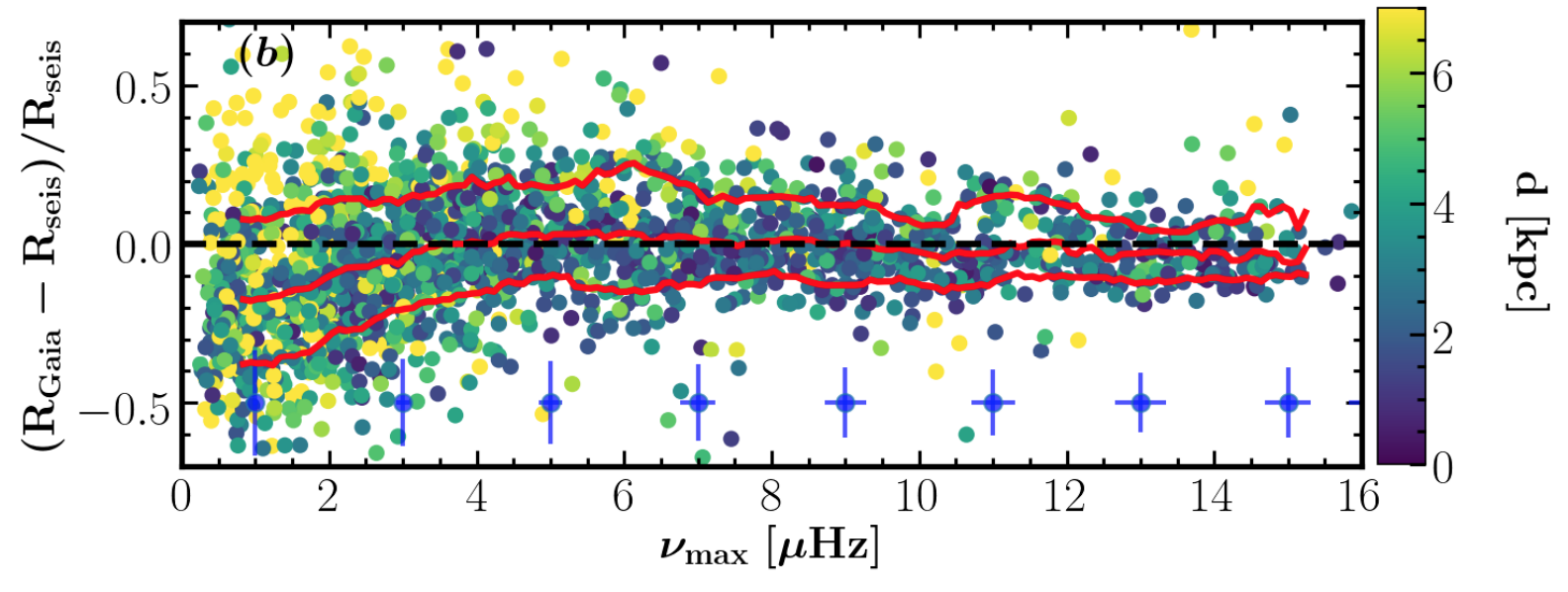
Figure 3: A comparison between stellar radius predicted by Gaia and predicted using asteroseismic scaling relations, coloured by distance to the star. The agreement is strong overall, but fails for stars oscillating slower than 3 microHertz. [Adapted from Figure 12 in the paper].
Typically, asteroseismology of solar-like oscillators uses scaling relations between observed oscillation properties of a star and those of the Sun, in order to determine a star’s mass and radius. But does this apply to these extreme fundamental-mode oscillators? By using data from the Gaia mission, they directly compared the star’s radius measured from its luminosity against a radius measured using asteroseismology. They found that the scaling relation was robust all the way down to frequencies of 3 microHertz (a 4 day period), but for stars oscillating slower than this it started deviating away, hinting at a possible change in underlying physics.
Finally, they looked at the amplitudes of the oscillations of different angular degree. For overtones of n = 3 and higher, they found that the dipole (l=1) modes were strongest, which is also typical for stars like the Sun. However at overtones of n = 2, the quadrupole (l=2) modes were strongest. Unfortunately this could not extend to the fundamental mode— to do so would require OGLE lightcurves with a baseline of 8 to 12 years!
Conclusions
Today’s paper is an excellent example of a deep dive into so-called ensemble asteroseismology, using large catalogues of oscillating stars to better understand their physics. These new revelations of how and why certain LPVs oscillate, along with more observations set to be made of such stars by the TESS mission, will allow astronomers to better understand the extreme physics of these highly evolved stars.