Title: Dynamic Zoom Simulations: a fast, adaptive algorithm for simulating lightcones
Authors: Enrico Garaldi, Matteo Nori, Marco Baldi
First Author’s Institution: Max Planck Institute for Astrophysics, Garching, Germany
Status: Submitted for publication in MNRAS
Cosmological simulations: valuable but expensive tools
Modern extragalactic astronomy and cosmology rely on numerical cosmological simulations. These simulations recreate the Universe in a computer. Matter is modelled by particles, either dark matter particles or baryons, set at initial positions given by the cosmic microwave background. The particles then move and interact according to a cosmological model and the hydrodynamical equations (for more details on hydro simulations, check out this astrobite). This way, theorists can try out many different models for physical processes, such as cosmological expansion and galaxy formation. By comparing the predictions of the simulations to actual observations, astronomers can figure out which models most accurately describe the Universe.
However, creating these simulations has a huge cost. They require significant computational time and memory. For example, one run of the IllustrisTNG simulation needed 90 million hours of CPU computing time, and its output is 128 TB large. To put this in context, a typical laptop hard drive can store 500 GB, so 256 laptops would be needed to store the total simulational output. The larger the simulated volume and the higher the required resolution, the more time and memory is needed to calculate and store the positions of the particles. It is therefore expensive to run many different large volume simulations in order to test many models, which will be needed to analyze future full-sky surveys like LSST and Euclid.
But don’t worry: the authors of today’s paper have an idea on how to address this issue. Their approach? Reducing the “waste” of cosmological simulations.
The wastefulness of cosmological simulations
Numerical simulations simulate many particles at unobservable positions. Given how expensive these simulations are, this is quite wasteful. Since light travels at a finite and constant speed c, we can only observe a source’s light emitted at time t if its distance from us is d=c*t. Such an object is on our “backwards light cone” —and we can infer information only about objects on our light cone, while the objects outside it are forever out of reach. The simulations, though, usually calculate and store the properties of particles in the whole volume at all times. Therefore, much of the information is not useful for comparisons of the simulation to the real world.
Figure 1 demonstrates this effect. The observer can only see particles that are on the solid line. If a particle is inside the light grey area, the observer will be able to see it at some point. However, if it is outside this area, the observer cannot see it anymore, it is too far away. The simulation, nevertheless, still calculates the full motion of all particles.
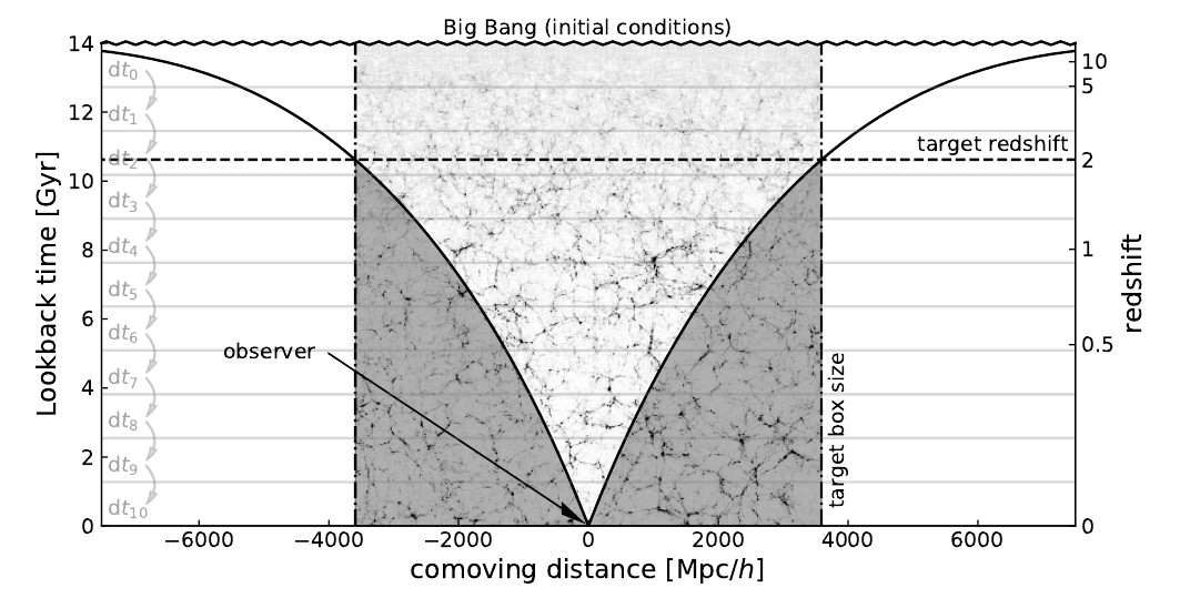
Figure 1: Illustration of the observable area of a simulation. The observer at time t=0 and position d=0 can see all particles on the solid line, which is the observer’s backwards lightcone. The shaded area corresponds to the simulational box. The observer can see objects in the light grey region at some point, but they can never see those that have entered the dark grey area. (Figure 1 in the paper)
So, if we cannot observe these particles outside of the lightcone, why not discard them completely? This approach is followed by some numerical simulation codes, for example, in the Euclid Flagship Simulation. However, this technique is not entirely correct, because, in the simulation, those particles that are outside of the lightcone can still influence the motion of particles inside the lightcone. Therefore, discarding them completely is problematic.
“Dynamical zooming” on what we actually want to simulate
The authors of today’s paper, therefore, follow a different approach. They keep simulating particles outside of the lightcone, but they lower the resolution in a method they call “Dynamical Zoom”.
After each time step, the algorithm looks at all the particles. If these particles are outside of the light cone and comply with a certain “de-refinement” criterion, they are merged with neighbouring particles. The next computational step then uses the merged object with the average position, speed, and mass of the original particles. The further away particles are from the light cone, the more particles get combined and the lower the final resolution. In this way, the volume outside the lightcone is still simulated but takes up much less memory and computational power.
The speed-up of this approach is impressive: Compared to a standard simulation, the computational time is reduced by 50%, and the authors expect even more speed-up for more complex or larger simulations.
But are the results reliable?
Of course, the speed-up of the simulation would be useless if the output would be dramatically different than the standard simulation. The authors, therefore, compare the matter density distribution in the two simulations.
Figure 2 shows the distribution of matter in the standard simulation and the simulation with Dynamical Zoom along with the fractional difference between the simulations. The two matter distributions are almost identical. The difference in the matter density is less than 0.15% at all positions. Furthermore, the number of dark matter halos predicted by the dynamical zoom simulation per halo mass agrees with the standard simulation within 0.02%. Consequently, the averaging of particles outside of the lightcone appears not to impact the scientific predictions of the simulations, while speeding-up the calculation immensely.
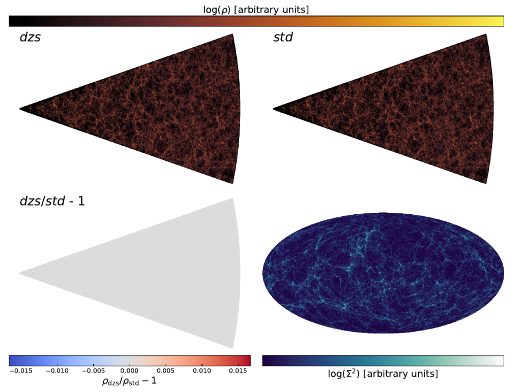
Figure 2: One slice of a simulated light cone. The upper plots show the matter density distribution ρ, either in the Dynamical Zoom Simulation (upper left) or the standard simulation (upper right). The lower left plot shows the fractional difference in the density between the two simulations. While this appears completely grey at first glance, there are minor differences (<0.15%) between the simulations on individual pixels. Consequently, the dynamical zoom method does not impact the predictions of the simulation. The lower right plot shows the projected matter density Σ of the Dynamical Zoom Simulation on the sky. (Figure 7 in the paper)
So, to summarize, dynamical zooming seems like a promising technique for future large-volume simulations of the Universe. It wastes less information than a standard cosmological simulation because only observable particles are simulated at high resolution, and is, therefore, faster and less memory-consuming. At the same time, its predictions are as accurate as those by standard simulations. Consequently, this technique might help create new cosmological simulations to be compared to observational surveys!
Author