Title: The Single-Cloud Star Formation Relation
Authors: Riwaj Pokhrel, Robert A. Gutermuth, Mark R. Krumholz, Christoph Federrath, Mark Heyer, Shivan Khullar, S. Thomas Megeath, Philip C. Myers, Stella S. R. Offner, Judith L. Pipher, William J. Fischer, Thomas Henning, Joseph L. Hora
First Author’s Institution: Ritter Astrophysical Research Center, Department of Physics and Astronomy, University of Toledo, Toledo, OH 43606, USA
Status: Accepted for publication in ApJL
Gas to Stars
Each of the many hundreds of stars we can see with our naked eye, or the many thousands we can see with the aid of telescopes, has their own special story of how they came to be. Now self-gravitating balls of gas, these stars in the night sky began as clumps in dense molecular clouds. Once these clumps become large enough, they gravitationally collapse and form stars. In our own galaxy, the Milky Way, we can study this process directly, and use the observations to infer much about its workings in more distant galaxies.
Since we know that dense gas is required to form stars, it is natural to ask what relationship there is between the two. In fact, the Kennicutt-Schmidt (KS) relation, tells us that there is a direct scaling between the mass of gas and the star formation rate (SFR). This relationship has allowed us to trace star formation throughout the history of the universe and understand how galaxies grow over cosmic time. But the authors of today’s paper asked a question that puts a slight twist on the KS relation: they wanted to know if such a relationship holds within individual molecular clouds.
Putting Clouds Under the Microscope
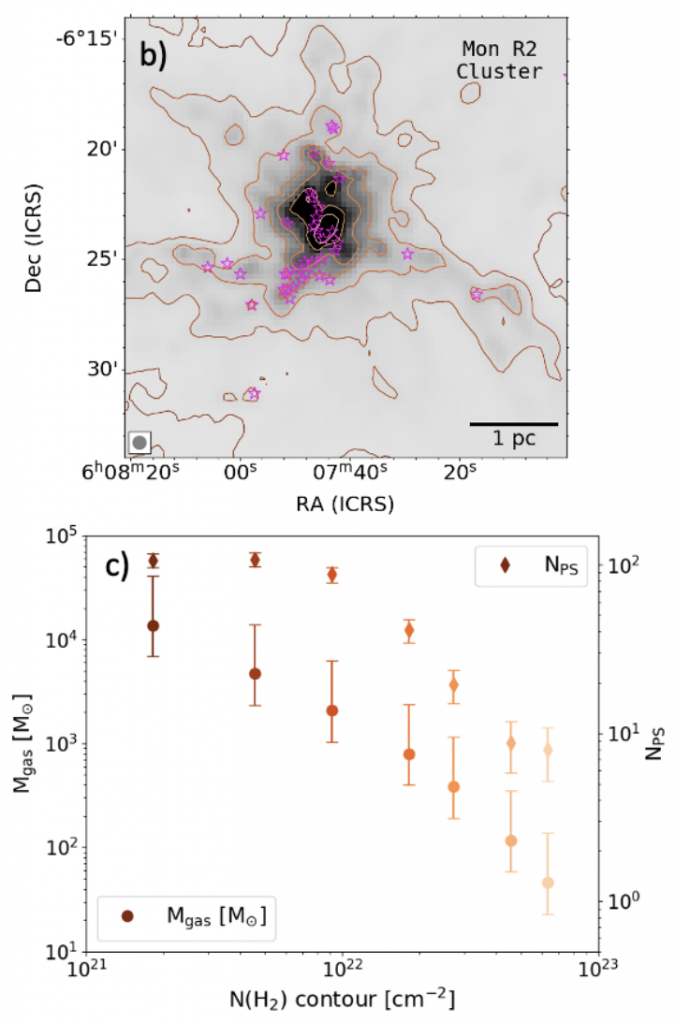
To answer this question, the authors used Spitzer and Herschel data for 12 well-studied star forming regions. Using the Herschel far-infrared data, they computed molecular hydrogen column density maps. With these measurements, they were able to compute the surface density of the gas in the star forming regions. With both near- and mid-infrared data from Spitzer the authors identified sources with a significant infrared excess and classified them into subclasses of young stellar objects (YSOs), also known as protostars. With these data, the authors measured the gas masses and number of stars within given density contours (corresponding to a physical area in the cloud). Figure 1 shows these values. From these, a gas surface density, a star formation surface density, and a free-fall timescale can be calculated. The authors assumed a stellar mass of 0.5 solar masses and a 0.5 Myr timescale to compute the SFR.
The Single Cloud Relation
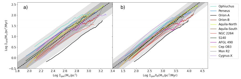
With measured gas and SFR surface densities, the authors were ready to answer their main question. Figure 2 shows the comparison of these two quantities. As can be seen, the SFR surface density and the gas surface density scale strongly with each other. In fact, when normalizing by the free-fall timescale (right panel of Figure 2), the scatter in the relationship is decreased and the relationship becomes linear, as expected from theory.
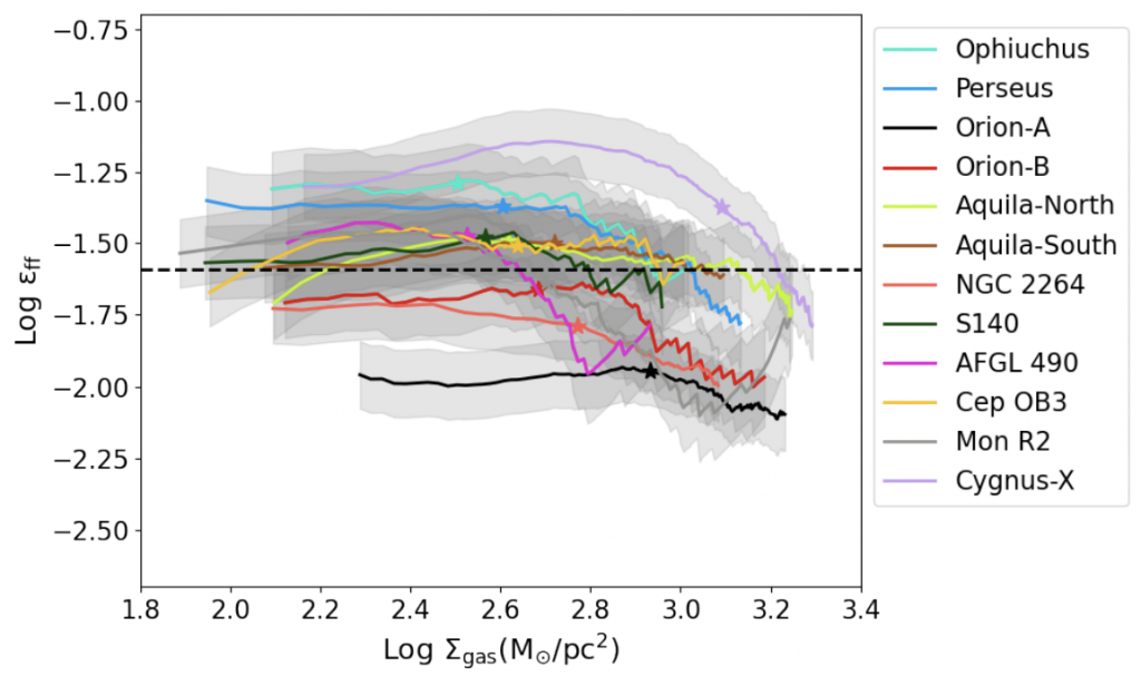
To further demonstrate that the relationship shown in Figure 2 is real and not due to the fact that both surface densities are area-dependent, the authors compare the gas surface density to the free-fall efficiency, which essentially measures how efficient the gas is at forming stars on a free-fall timescale. This comparison is shown in Figure 3. With no clear global trend between the free-fall efficiency and the gas surface density, the authors are confident that their single cloud star formation relationship is valid.
In summary, the authors of today’s paper have shown that the KS relation that has been used for years in extragalactic studies has a local analog. This is particularly interesting as the various clouds in their sample have a wide range of physical properties. This correlation implies that star formation is regulated by processes on small scales, including stellar outflows or turbulence, rather than galaxy-scale effects such as supernovae and galactic properties. As we continue to study star formation in greater detail, the deeper meaning of this correlation may give us even deeper insights into how the stars we see every night were born.
Astrobite Edited By: Suchitra Narayanan
Featured Image Credit: NASA