Title: Autoencoding Galaxy Spectra I: Architecture
Authors: P. Melchior, Y. Liang, C. Hahn, et al.
First Author’s Institution: Department of Astrophysical Sciences, Princeton University, NJ, USA and Center for Statistics & Machine Learning, Princeton University, NJ, USA
Status: Submitted to AJ
Imagine for a moment that you’d never seen a car before and you really wanted to build a toy car as a gift for a car-loving friend of yours. Understandably, faced with this conundrum, you might feel that the outlook is bleak. However, now suppose that another friend came along and had the bright idea to send you to the nearest busy street corner, explaining that everything passing by can be considered a car. They then bid you adieu and depart. Armed with this new information, you are reinvigorated. Watching the vehicles pass by for a few minutes, you quickly form an image in your mind of what a car might be. After about an hour, you head back inside, ready to take on your challenge: you need to build your own (toy) car based only on what you saw.
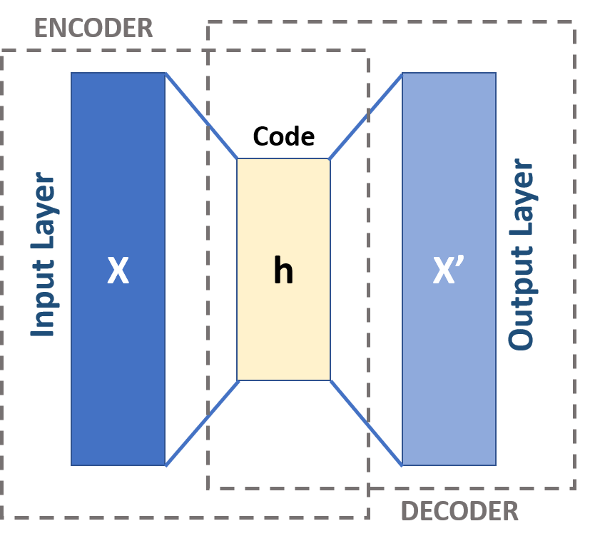
This example is obviously contrived but provides a useful touchpoint from which we can heuristically understand how an autoencoder, or, more generally, any unsupervised machine learning algorithm, might work (see these astrobites for examples of machine learning used in astronomy). If you think about how you’d approach the above challenge, the basic principle might be clear: with only the observations of the cars passing by, you’d latch onto patterns that you noticed and use those to “reconstruct” the definition of a car in your mind. Perhaps you’d see that most of them had four wheels, many had headlights, and they all had generally the same shape. From this, you might be able to construct a decent looking toy car and your friend would be proud. This is the basic idea behind an unsupervised learning task: the algorithm is presented with data and it tries to identify relevant features of that data to assist with some goal that it has been presented. In the specific case of an autoencoder, that goal is to learn how to reconstruct the original data from the compressed dataset, as you were attempting to do by building a toy car from memory. In particular, you (or the computer) are boiling down the observations of the cars (the data) into shared characteristics (the so-called ‘latent features’) and rebuilding the car from those characteristics (reconstructing the data). This process is depicted schematically in Figure 1.
Applying this to astronomy
To understand how this machine learning method is applied in today’s paper, let’s take the example of the car reconstruction one step further. Rather than being able to observe a random sampling of cars driving by, this time let’s say your friend was less ingenious and just pulled up pictures of a few different cars on their phone. Based on this, you might be able to do a decent job at producing something that looks like a car, but your car likely wouldn’t work too well (e.g., perhaps the wheels would be attached to the chassis and your car wouldn’t move). Alternatively, maybe your friend wanted to challenge you further and just described how a car works. In that case you might be able to build a decently functional toy car, but it probably wouldn’t look too accurate. These scenarios are loosely analogous to some of the challenges present in current approaches to modeling galaxy spectra, the subject of today’s paper.
The approaches to modeling galaxy spectra can be split between the empirical, data-driven models and the theoretical models. The former of these are equivalent to the pictures of cars your friend showed you — astronomers use ‘template’ spectra and observations of local galaxies to construct model spectra that can be fit to observations of systems at higher redshifts. While useful, these are usually based on observations of local galaxies and may therefore be restricted to a limited wavelength range once the cosmological redshift correction is incorporated. The theoretical models, on the other hand, mirror the latter suggestion from your friend; namely, they produce model spectra based on a physical understanding of the emission and absorption in the interstellar medium, in stars, and in nebulae. These are interpretable and physically motivated, so can be applied to higher redshifts, for example, but usually rely on some approximations and are therefore not able to capture the complexity of true spectra accurately.
Despite these challenges, today’s authors note that the historical utility of applying template spectra to describing new observations of other spectra implies that this data may not be as intrinsically complicated as it appears — perhaps the variations between spectra can be boiled down to a few relevant parameters. This harks back to the discussion around autoencoders and inspires the approach of today’s paper — maybe one can find a low-dimensional embedding (read: simpler representation) of the spectra that makes reconstruction an easy task.
How to build a galaxy spectrum
Most traditional galaxy spectrum analysis pipelines work by transforming the observed (redshifted) spectrum to the emitted spectrum in the rest frame of the galaxy and then fitting the observation to a model. This means that the spectra are usually limited in the usable wavelength range to a range that is shared between all the different spectra in a survey sample. In today’s authors’ architecture, they choose to keep the spectra as observed, meaning that they do not do any kind of redshift processing prior to their analysis, allowing them to present the algorithm with the entire wavelength range of the observation, thereby preserving more of the data. Today’s paper presents this algorithm, called SPENDER, which is schematically represented in Figure 2.
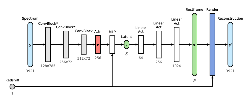
The algorithm takes an input spectrum and first passes it through three convolution layers to reduce the dimensionality. Then, because the spectra have not been redshifted, the processed data is passed through an attention layer. This is very similar to what you would be doing when watching the cars pass by on the street — though there were many cars passing by and they were all at different locations and moving at different speeds, you focused your attention on particular cars and particular features of those cars to train your neural network (read: brain) to learn what a car was. This layer does the same thing by identifying which portions of the spectrum it should focus on; i.e., where the relevant emission and absorption lines may be. Then, to conclude the encoding of the data, the data is passed through a multi-layer perceptron (MLP) that redshifts the data to the galaxy rest-frame and compresses the data to s-dimensions (the desired dimensionality of the latent space).
Now the model has to decode the embedded data and attempt to reproduce the original spectrum. It does this by passing the data through three ‘activation layers’ that process the data through some preset function. These layers transform the simple, low-dimensional (latent) representation of the data to the spectrum in the galaxy’s rest frame. Finally, this representation is redshifted back to the observation and the reconstruction process is complete.
In practice, the contributions of various parts of the data to the final result depend on weights that are initially unknown. To learn these weights, the model is trained — the reconstructed and original data are compared and the weights are tweaked (roughly by trial and error) until the optimal set of weights is achieved.
So how does it do?
The results of running the SPENDER model on an example spectrum from a galaxy in the Sloan Digital Sky Survey are given in Figure 3.
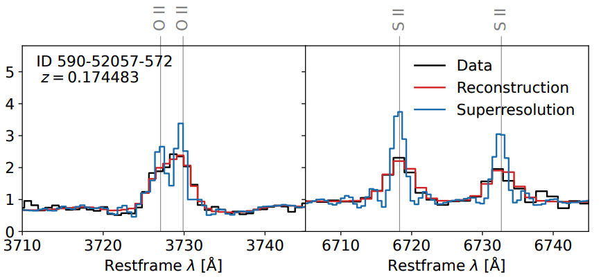
Visually, it appears that the model does quite well at reproducing the given spectrum. Figure 3 also demonstrates one of the advantages of a model such as this. Not only is the model able to reproduce the various complexities of the spectrum, but by varying the resolution of the reconstructed spectrum, the model is able to distinguish features that are overlapping (or blended) in the input data (see the two nearby OII lines in Figure 3, for example). Ultimately, the nature of the SPENDER construction means that data can be passed to the model as it is received from the instrument — because the model is trained with no input redshifting or cleaning, the model learns to incorporate that processing in its analysis. Such an architecture can also be used for generating mock spectra and provides a new approach to modeling galaxy spectra in detail that mitigates some of the issues that exist in current empirical galaxy modeling approaches.
Astrobite edited by Katy Proctor
Featured image credit: adapted from the paper and bizior (via FreeImages)