My name is Eunhee Ko, and I am a graduate student at Seoul National University studying the connection between galaxy clusters and their surrounding large-scale structures, as well as their co-evolution. In my free time, I enjoy taking pictures with film cameras and find that the process of capturing a moment in time through a lens parallels my work as an astronomer.
Title: Clustering-based redshift estimation: comparison to spectroscopic redshifts
Authors: Mubdi Rahman, Brice Ménard, Ryan Scranton, Samuel J. Schmidt, Christopher B. Morrison
First Author’s Institution: Johns Hopkins University, Baltimore, USA
Status: Published in MNRAS, Jan. 2015
Can you extract the 3D information from 2D?
Measuring distance to astronomical objects is the most important task for astronomers. Also known as Cosmic distance ladder, determining distances accurately enables us to probe the universe’s evolution in various epochs. The concept of redshift, defined as how an observed galaxy’s wavelength is shifted from the rest-frame, can act as a distance indicator, although it is unitless, unlike usual length quantities. By calculating the wavelength shift ratio, which results from the cosmic expansion, we can successfully estimate how the galaxy is far from us.
To obtain the reshift, astronomers can observe a galaxy’s spectrum. The spectroscopic redshift is accurate but this process requires a lot of time and cost. On the other hand, we can alternatively estimate it with comparison of fluxes from photometric bands and template spectral energy distribution (SED), so-called photometric redshift. The photometric redshift method is relatively cheap in terms of observational time and cost, however, its errors are too large to resolve the cosmic structures reliably. To be specific, overlapping structures such as galaxy clusters and groups might seem located in the same distance while they are actually separated. As a result, there are trade-offs between the measured redshift’s reliability and expenses for observations.
Here the motivation for clustering-based redshift estimation comes up. With the groundbreaking technique, we estimate the redshift only from Right Ascension (RA) and declination (dec) with reference spectroscopic samples. In other words, we can derive redshift information only from 2 dimensional coordinates.
Voilà! Cross correlation function can do it!
Before diving into it, we need to understand the role of a cross correlation function. Simply put, the cross correlation is the spatial distribution of galaxies in the universe. It can describe how two or more galaxies are far away from each other and calculate their distribution’s probability based on the cosmological evolution. In this regard, the underlying idea of the clustering-based redshift estimation is that the derived cross correlation from the galaxies with known redshift allows the inference of a galaxy’s unknown redshift. If two galaxies are overlapping in redshift, then their angular correlation is likely to be higher while lower if not. Therefore, nearby counterparts in the transverse distance are more probable to be connected to each other. Note that this method is reliable only when the reference samples and their distribution are well defined. Otherwise, it will lead to wrong outcomes.
For practical implementation, we need two samples: a reference population and an unknown population. A reference population consists of extragalactic objects whose both angular positions and redshifts are known. The other unknown population does not include redshifts, but only angular positions. From the cross correlation from the reference population, we can determine the probability distribution of redshifts in the unknown population. Actually, this approach was first proposed by pioneering astronomers, Seldner and Peebles in 1979, and has been continuously developed by several researchers. After the beginning of the 21th century, burgeoning photometric surveys over a large area ultimately made it possible to try its actual utilization.
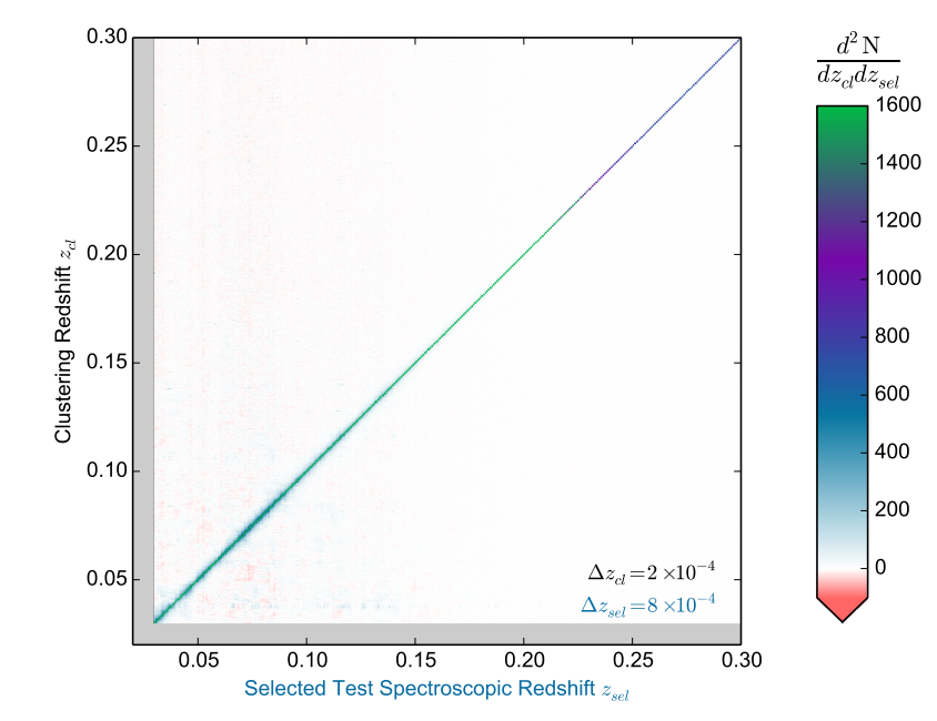
The authors in this study test the validity of this method by using the Legacy Spectroscopic Sample from the Sloan Digital Sky Survey data. After limiting the r-band magnitude to 19 mag and removing unreliable data such as poor photometry, sky background etc, they measured spatial cross-correlations between 0.03 < z < 0.3. Surprisingly, the clustering-based redshift and spectroscopic redshift are in a good agreement. According to figure 1, more than 90% of the sample galaxies are consistent with the spectroscopic redshifts.
Takeaways: remaining problems and solutions
Still, there are controversies about the reliability of the method and it is thereby necessary to obtain the spectra for confirmation. If a massive galaxy cluster is present in the reference sample, this will create a falsely derived strong correlation in horizontal direction and disrupt the cross correlation function. Moreover, the radial motion of a galaxy results from the Hubble flow and peculiar velocity. This effect is stronger when massive structures such as galaxy clusters are close enough. It is also possible that superpositions of cosmic structures in different redshift spaces generate an artificial correlation. The mentioned contaminations remain to be solved in the future analysis.
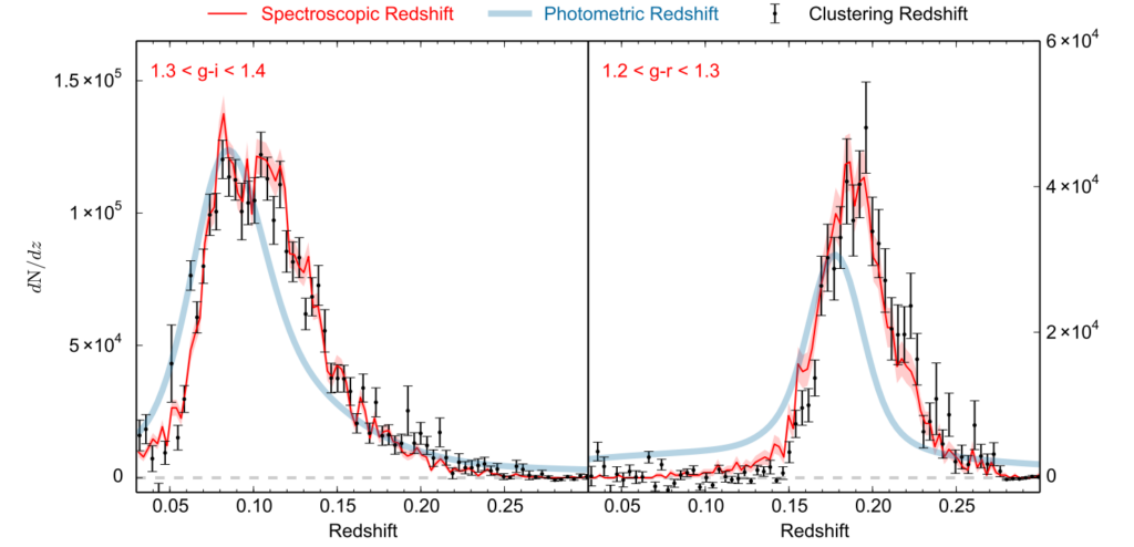
Despite its limitations, we can make use of the clustering-based method in preparation for the future survey. For example, astronomers validate their photometric redshift estimates with the clustering redshifts. Figure 2 describes the number distribution as a function of redshift. The overall prediction from the clustering-based estimations is a greater match with spectroscopic observations than the photometric redshift. With the aid of upcoming surveys and advanced analysis, we hope to probe the universe more precisely!
Astrobite edited by Jessie Thwaites