The Undergraduate Research series is where we feature the research that you’re doing. If you are an undergraduate that took part in an REU or similar astro research project and would like to share this on Astrobites, please check out our submission page for more details. We would also love to hear about your more general research experience!
by Yash Gondhalekar
Birla Institute of Technology and Science, Pilani
This guest post was written by Yash Gondhalekar. Yash is a recent graduate in Computer Science from the Birla Institute of Technology and Science, Pilani. He completed this research during his final year of undergraduate under the supervision of Prof. Eric Feigelson, partly done during his undergraduate thesis. A preliminary version of the work was presented at AAS241 and was accepted for publication in the Astrophysical Journal Letters (arXiv preprint).
The transit method is the most widely used method to detect exoplanets. While it is relatively easier to discover large-sized planets (e.g., Jupiter-sized), detecting small, Earth- and Mars-sized transiting planets poses several difficulties since factors such as intrinsic stellar variability, instrumental effects, and red and photon detector noise can make distinguishing faint transit periodic dips from these factors difficult. Thus, each step during detection must be carefully handled, which requires sound statistical approaches.
In a typical transiting planet detection pipeline, the stellar light curve is first detrended to remove non-periodic variations unrelated to the transit dips, such as stellar variations. Periodograms are constructed using the detrended light curve to search for possible periodic dips. Typically, the highest peak in the periodogram is examined for its significance – whether the observed peak arises due to a possible transit signal or random fluctuations in the time series due to noise.
Several common choices for detrending exist, e.g., Splines, Gaussian Processes Regression; the False Alarm Probability (FAP) and the Signal-to-Noise Ratio (SNR) of the periodogram peak are two popular significance measures; and the most common choice for the periodogram is the Box-Least Squares (BLS) algorithm (Kovacs et al., 2002). However, traditional detrending approaches are meant to remove long-term trends, so short-memory autocorrelation (primarily due to stellar activities) remains mostly unaddressed. This was shown in Figure 5 of Melton et al., 2023b, where ~36% TESS light curves possessed significant short memory correlation after detrending by Splines.
In this study, the authors show two exciting results:
- The BLS periodogram becomes incompetent if the autocorrelation is not effectively removed from the light curve – the autocorrelation can closely mimic a transit-like shape, fooling BLS into believing that the autocorrelated noise is a true box-like transit!
- An effective treatment of the short-memory autocorrelation: AutoRegressive Integrated Moving Average (ARIMA) modeling, if followed by the (relatively unknown) Transit Comb Filter (TCF) periodogram (Caceres et al., 2019a), can improve sensitivity to small planets compared to BLS.
The experimental procedure is as follows: to understand periodogram behaviors in different noise patterns, they simulate two types of light curves containing transits: pure Gaussian and AutoRegressive Moving Average (ARMA) noise. The transit depth is varied while keeping all other planetary parameters unchanged (e.g., planetary period, transit duration). The FAP and SNR significance measures are applied to the periodograms for each simulated depth. The depth at which the planet was barely detectable is calculated (i.e., the lowest depth satisfying FAP < 0.01 or SNR > 6), called the Minimum Detectable Depth (MDD). MDD is then calculated for different numbers of transits in the light curve, resulting in a plot in Figure 1. The Gaussian Processes Regression detrender is used before BLS.
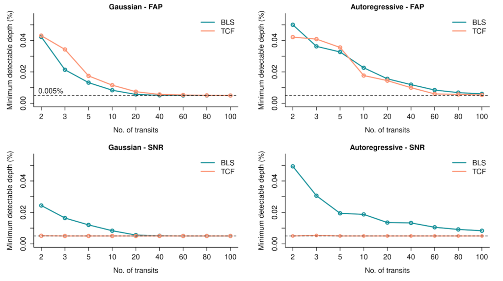
Since the ultimate goal is to detect small planets reliably, the authors ask what periodogram and significance metric combinations yield the lowest MDD in general. The figure suggests it is the TCF – SNR combination. Thus, the authors suggest one should use the TCF periodogram rather than the BLS periodogram and use the SNR detection metric on the periodogram peak to detect smaller planets than possible with the current standard method, BLS. Surprisingly, the figure shows that even in pure Gaussian noise, TCF has better SNR than BLS; consequently, its MDD was lower than BLS. TCF was, however, found to be less sensitive than BLS using the FAP criterion when too many transits are not present in Gaussian noise.
Both BLS and TCF give near-optimal sensitivity (using both FAP and SNR) if sufficiently many transits (≳ 30-40) are present in Gaussian light curves, so the choice of the periodogram, only in this case, would not matter. But this pattern is not observed for Autoregressive noise where TCF is better than BLS even with many transits such as 60-80. The application to four real TESS light curves (with mild autocorrelation) agreed with their simulation results.
For (2), the authors considered simulated Autoregressive light curves and manually selected two false peaks in the BLS periodogram. They visualized the BLS box fits corresponding to the planet periods associated with the false peaks. A visual inspection suggested that the BLS fits a box to an autocorrelated structure that is not a transit signal!
Overall, ARIMA combined with TCF is more sensitive than BLS. Thus, the authors strongly encourage users to consider replacing BLS with the ARIMA + TCF pipeline not only when autocorrelation is present in the light curve after detrending but also when the detrended light curve has Gaussian noise. Another reason to use TCF is its much better noise characteristics (smaller heteroscedasticity and trends in periodogram powers) than BLS (Ofir, 2014).
The described comparison approach is versatile, so it can be extended to compare any periodogram algorithms and select the better-performing periodogram. An intriguing idea is to compare BLS with its astrophysics-informed variant, Transit Least Squares (TLS) (Hippke & Heller, 2019). This study could have potential applications in upcoming transiting exoplanet surveys and help improve current detection capabilities.
Astrobite edited by: Ali Crisp