Authors: Bjoern Benneke and Sara Seager
First Author’s Institution: MIT
Paper Status: Accepted to ApJ, 2012
“Atmospheric retrievalists” are the middle child of exoplanet studies. The exoplanet saga usually goes as follows: A group of astronomers observe planet X for _____ hours and get fantastic data! Theorists agree that this planet could be ______. In this rendition of story there are two groups of people doing the work: the observationalists and the theorists. Here is where the problem comes into play. There is a whole other branch of exoplanet studies that actually builds the bridge between what we observe and what we model. Sadly, there have been no astrobites to date, on any of these techniques. Therefore, in today’s astrobites I would like to take some time acknowledge the work that has been done in this field by a relatively old paper by Benneke & Seager.
When I talk about exoplanet studies, I am specifically talking about characterization of different planetary atmospheres. Take for example GJ 1214 b and WASP 12b. In both these cases, observers studied them in transit to get relatively good transmission spectroscopy of their planetary atmospheres. But, the long-standing question is: what information about the planet can you get out of these transmission spectra? If you were looking at individual absorption features of certain gases, you would certainly be able to ascertain something about what gases are present in the atmosphere. However, what if you want to probe deeper than that? It’s much more useful to ask not only if you could tell if a gas was present in an atmosphere but also if you could tell how much of the gas was present. If there was methane in hypothetical Planet X, is there 40% methane or only 1% methane? It is here where the work by Benneke & Seager becomes crucial. In order to uniquely constrain these planetary atmospheres they follow this procedure:
- Analyze all of your spectral features
- Decide what parameters you are interested in recovering
- Produce millions of models with those parameters
- Decide which best fit your data
When put like this, it seems natural that the retrievalist often becomes the middle child. Let’s be honest, no one is interested in spending too much time on the statistical analysis of a paper. Almost 100% of the time, you care about the observation and the results. But, this four-step process is all but a simple one. So, it behooves us to go through it step by step and carefully understand what assumptions are going into the work.
Analysis of spectral features
Below is a model of an exoplanet transmission spectrum for a mystery planet X. In reality, our observations don’t look nearly as good as these models (yet) but this tells us what features we need to measure when deriving planet properties from transmission spectra. The first thing you’ll notice is the amount of features that are needed in order to get absolute mixing ratios.
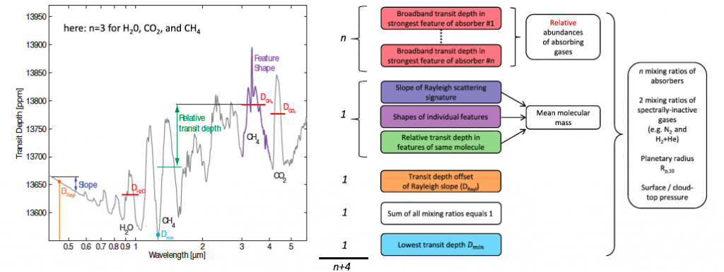
On the left, is an example transmission spectrum of a planetary atmosphere. Labeled, are specific features that are important for atmospheric characterization. The diagram on the right shows how these spectral features combine to give you different planetary parameters.
For reference, I would take a look at the WASP 12b observation where they observed a single water feature from 1.1 to 1.7 micron. In that study though, they were able to get an approximate mixing ratio for water, which completely disagrees with the figure you see above. The difference here is that Benneke & Seager are trying to build an atmospheric retrieval technique that will work on not only gaseous planets, like WASP 12b, but also super Earth planets like GJ 1214b. The subtlety, therefore, lies in what you assume is the dominant constituent of your atmosphere. Gaseous planets like Jupiter have huge surface gravities so they can retain massive hydrogen-helium atmospheres. Smaller planets can’t hold on to the hydrogen and helium and end up with much smaller atmospheres made up of a heavier gas. Earth, for example ended up with mostly nitrogen and Venus ended up with mostly carbon dioxide. Therefore, if you know you are looking at a gaseous planet, you can assume it’s mostly hydrogen and helium. This is why for WASP 12b, they were able to get an approximate water abundance even though they didn’t have access to all the features outlined in that first figure.
Knowing this information, let’s take a look at figure one again. Because you don’t see any hydrogen features and you don’t see any nitrogen features you might be inclined to say that our planet X is dominated by carbon dioxide and methane. Sadly, this would certainly lead you down the wrong path since nitrogen and hydrogen are what we call “spectrally inactive gases”. Meaning, although they don’t appear in the spectra, they might still be there and might still be making up most of the atmospheric component! This is a striking fact and it does not bode well for us in terms of trying to figure out what these planetary atmospheres are made of. This is why we need so many spectral features to get any planet information at all.
What Parameters to Recover
This is a philosophical question along with scientific one. Technically, you would like to recover as much information as possible about these exoplanets. But, at what point do you draw the line? These exoplanet atmospheres only offer us a small peak into what is happening to the planet as a whole. Therefore, our models must retain a certain level of simplicity so that we are not “over-fitting” any of our features. For example, let’s say someone blind folded you and asked you to determine the composition of a bite of food. If you have a nice taste pallet, you’d probably be able to determine bulk ingredients: chicken, carrots, peas, etc. If you are an expert you might be able to say something along the lines of: 80% chicken, 10% carrots, 10% peas. If you tried to then determine how the chef spent his time preparing the dish, that might be a stretch. At that point, we would say you are putting too much weight on just that one bite you took, and are therefore “over-fitting” the data. In their model, Benneke and Seager determine that the parameters we can get from planetary spectra are the following:
- Volume mixing ratios of atmospheric constituents: i.e., planet X is 99% hydrogen, 0.5% carbon dioxide, 0.5% nitrogen.
- Surface or cloud deck pressure: i.e., planet X has a surface pressure of 1 bar, like Earth. Or maybe, we can’t see a surface at all! Instead, we are looking at a thick layer of clouds with a pressure of 0.001 bars!
- Planet radius:e., if planet X does have a very high cloud later, where is the surface?? Or, if the planet has no surface at all (like a gaseous Jupiter planet) where do we define the deepest atmospheric layer?
- Planetary albedo: i.e., how much light is planet X absorbing, versus reflecting
Modeling Thousands of Spectra and Statistics
In order to pin down these four parameters, we need to find the most exact combination of parameters that fit the spectrum of planet X. And as you might imagine, trying to guess what those might be is worse than trying to guess lottery ticket numbers! So the only way to make it work is to try thousands of times! Benneke & Seager generate about 100,000 of these models before they actually can move on to their statistical analysis. Now you can appreciate why it’s so sad that the atmospheric retrievalist get forgotten about! Once 100,000 models have been created, each model is carefully compared to the spectrum of planet X (the data) in order to determine a best match. This is done through very complicated statistical models which a guest writer Ben Nelson did a wonderful job of explaining in this post. In the spirit of completeness I’ll give a short summary here.
The basic principle is to start with four initial conditions for your four parameters and calculate the probability that those are correct. Chances are they will not be… So we jump to another combination of those four parameters and test those out. Is the probability of those four parameters being correct higher than your initial guess? If not, go back to your initial guess and try again. A great analogy for this, is the idea of climbing up a mountain. You start at the bottom of the mountain with very low probability of being correct and your goal is to make it to the very top. In some cases, you might accidentally choose a path that will lead you down the mountain. But if you evaluate your altitude (i.e. your probability) at regular intervals you would hope to make it to the top as fast as possible. The same idea applies here to the idea of picking four correct parameters in a sea of an almost infinite number of choices.
The last figure I will show is this pyramid like structure that appears at the end of Benneke and Seager’s work. Each leg of this pyramid is the mixing ratio of a different type of gaseous species: oxygen, carbon, nitrogen and hydrogen/helium. Therefore, it’s a great insight into the amount of parameter space we are dealing with (remember that getting mixing ratios is just one of the four parameters we are trying to fit). But more importantly, it gives us insights into what can be gained from these retrieval techniques. Here, they’ve fed three different “pretend” observations through their retrieval technique: one hot-neptune like planet (green), one nitrogen rich planet (red) and one methane rich planet (blue). You can see by the very distinct groups of dots, that you can really tell the difference between these planets with this complicated retrieval technique. This is a great sanity check.
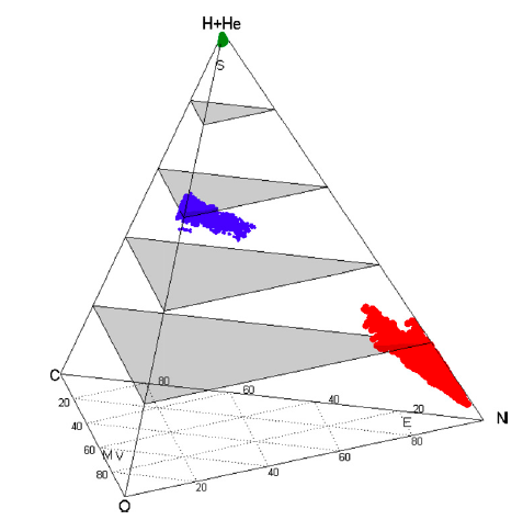
This pyramid like structure is called a quaternary diagram. It illustrates a large range of parameter space for different gaseous species: hydrogen/helium, nitrogen, carbon and oxygen. The different groupings of points show the retrieval results for three different planets. The fact that they are grouped in very different regions shows that we could theoretically tell the difference between these three kinds of planets: hot and neptune like planet (green), hot methane rich planet (blue) and hot nitrogen rich planet (red). Main point: atmospheric retrieval works!!
The study of exoplanet atmospheres will take off with launch of the James Webb Space Telescope and it is so important that the technique for retrieving planetary parameters from spectra works well! Without them, we have no way of testing our theoretical models against the real data. So even though retrievalists are the middle child of exoplanet characterization, we should really spend some time taking note of what they are doing!

Thank you for pointing out the need for middle-ground analysts between pure observation and hypothetic model building, Natasha. We have the same issue in molecular cloud / star formation analysis. Loads of data on one side and loads of plausible hand-waving on the other. There are fewer applied physics analysts than could be desired and I do wish I could see more hair on the floor from Occam’s Razor applied to model-building. The applied physics papers that carry the most weight the longest are those in which the equations become very simple and yet cover both observation and model. There seems to be a time lag of 10 or 15 years between the juxtaposition of a new data sets (e.g. turbulence and ambipolar diffusion, or shear tensors in cosmic sheets) until the bewildering maths terms that emerge from the resulting equations refine into coherent simplicity. Today, just as we thought we had diffusion/turbulence under our belts, along come younger authors exploring relationships we hadn’t though of before—e.g., column density of star formation as a PDF function of the Mach number of turbulence pockets in star-forming cores. I take these new papers outside and gaze up at an object we all know well, and it dawns on me, “This stuff sounds nuts . . . but it’s right.”
FWIW, I have not seen the equivalent of your quaternary diagram used in studies of molecular cloud structures. Could you send along some of the papers / authors that detail how these are diagrams populated and the data transformed into 3-D space?
Cheers, Doug Bullis in S Africa