Authors: Kevin Heng, Daniel Kitzmann
First Author’s Institution: University of Bern, Center for Space and Habitability
Status: Accepted to MNRAS, open access
Transmission spectroscopy is the most commonly used method to characterize the atmospheres of transiting exoplanets that have been discovered to date. The method is seemingly straightforward: photons from the host star passing through the limb of its transiting exoplanet are absorbed or transmitted by the planetary atmosphere to a varying extent in different wavelengths, which should appear as a variation in observed radius of the exoplanet with respect to wavelength. This variation in transit radius with wavelength, known as transmission spectrum, can then be interpreted by adopting either a forward or inverse modeling approach. This means that you can either start with a set of assumptions for the atmospheric properties (like chemical abundances, cloud properties etc.) and construct a physical model that can be fit to the data, or try solving the inverse problem (also known as retrieval) and infer the atmospheric properties from the measured transmission spectra itself.
However, there is a good deal of subtlety behind both approaches of constructing theoretical models for transiting exoplanet atmospheres. Today’s paper traces the assumptions and caveats involved in constructing models for observations taken by the Wide Field Camera 3 (WFC3) on the Hubble Space Telescope. In addition to deriving a validated semi-analytical approach from first principles for calculating the transmission spectra in the context of WFC3 observations, authors of today’s paper uncover a crucial and unresolved degeneracy involved in fitting a model to the transmission spectra.
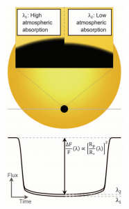
Figure 1: Variation in transit depth of a transiting planet due to wavelength dependent opacities of chemical species present in the planetary atmosphere (from de Wit and Seager (2013)). The inferred value of planetary radius Rp in units of the radius of the star as a function of the wavelength is the transmission spectra.
A crash course in transmission spectroscopy calculations
An important quantity of interest when trying to describe an atmosphere is its pressure scale height (H) – the scale at which pressure decreases exponentially with height in the atmosphere. It can be expressed as the ratio of the thermal energy of the gas molecules in the atmosphere to their gravitational energy, and can be expressed as kT/mg for an isothermal atmosphere (one that can be described by a single temperature T), mass of a molecule m, and surface gravity g (k is the Boltzmann constant). This ratio actually comes in as a natural consequence of assuming an ideal gas behavior (no interactions between gas molecules except collisions) and hydrostatic equilibrium for the atmosphere.
The exponential variation in pressure with height is associated with an exponential decrease in the number density of gas molecules in the atmosphere and this, along with the opacity (cross-section per unit mass) of the gas molecules, can inform us about the optical depth (ratio of incident to transmitted power of radiation by a medium) of the atmosphere at different heights. A change in the optical depth with respect to height causes a change in the amount of stellar radiation that is absorbed in different altitudes. On top of this, wavelength dependent opacities of gas and aerosol particles in the atmosphere introduce a variation in the amount of stellar radiation absorbed (and hence the apparent radius of the planet) with respect to wavelength as shown in Figure 1., and this gives you the transmission spectrum.
Effectively the shapes of the features in transmission spectra are controlled by a combination of pressure scale height and opacity (which also depends on the abundance of the corresponding absorbing species in the atmosphere). This can help us in inferring the abundance of the absorbing chemical species in a planetary atmosphere, the most significant of which is water for hot-Jupiters in the context of the wavelength range of 1.1 to 1.6 μm probed by HST/WFC3. However, to normalize the model transmission spectra used for fitting the observations, you need to assign a reference pressure for the chosen value of reference transit radius. As today’s authors, Heng & Kitzmann, point out, this is not always consistently possible and will generally lead to a degeneracy in the interpretation of transmission spectra.
Reference pressure or reference radius or water abundance?
The observed transit radius R as a function of wavelength that constitutes the transmission spectra can be written as R = R0 + h, where R0 is reference radius usually pegged to that obtained from the “white” transit light curve (time series photometry of the transit integrated over the whole wavelength range) and h is the effective thickness of the atmosphere that contributes to the absorption of stellar radiation. Using concepts of radiative transfer and assuming a high optical depth at R0, Heng & Kitzmann derive an expression for R for both isothermal and non-isothermal atmospheres. For the isothermal case (which provides fits comparable to that from non-isothermal expression as tested by the authors), this takes the analytical form: R = C + H logκ, where H is the isothermal pressure scale height, κ is the opacity (proportional to the abundance (χ) of the corresponding absorbing species like water), and C is a constant that contains a combination of R0 and P0 (reference pressure at reference radius value R0). The degeneracy between R0, P0, and χ immediately becomes apparent from this expression for transit radius when the authors try to fit it to the transmission spectra of hot Jupiter WASP-12b measured by HST/WFC3 (see Figure 2).
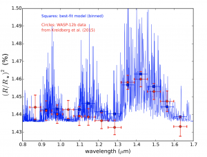
Figure 2: Best-fit Isothermal analytical model (in blue) for transmission spectra for the WASP-12b observations from HST/WFC3 (shown in red).The vertical axes shows the ratio of planetary radius to stellar radius as inferred from the depth of a transit light curve .(Figure 6 in the paper).
The reference pressure P0 in the analytical expression actually appears with χ as log(χ P0), while R0 appears linearly. In essence, this means small changes in R0 when trying to fit the same data will lead to orders of magnitude change in the inferred abundance χ (actually the inferred value of the product χ P0), as shown in Figure 3. Thus unless we know an exact functional relationship between R0 and P0, it’s not possible to conclusively break this degeneracy.
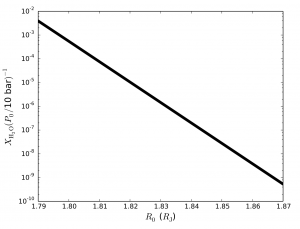
Figure 3: This shows the variation in the inferred value of water abundance from the best fit model for WASP-12b observations with respect to different assumed values of reference radius R0 (shown here in units of Jupiter radii RJ). Note that change in the reference radius value by few percents leads to orders of magnitude change in the inferred water abundance value from the model. (Figure 7 in the paper).
All may not be lost: possible workarounds
The authors further discuss special scenarios in which this degeneracy may be averted. Considering only the geometric mean opacities of all absorbing species can give an approximate relation between R0 and P0, but that is correct only at an order-of-magnitude level. In other cases, if you are in luck and come across a cloud-free hot Jupiter, stronger signatures of Rayleigh scattering (scattering of radiation by particles smaller than the wavelength of the radiation) can be used to associate a reference radius value with the pressure level being probed by the observations. Nevertheless, this degeneracy revealed by today’s paper just adds to the already existing degeneracies in exoplanetary atmosphere models due to clouds and hazes. It would be interesting to see how the next generation of exoplanet observations from the James Webb Space Telescope and simultaneous advances in modeling might help in alleviating some of these degeneracies and let us obtain more reliable constraints on the abundances of exoplanet atmospheric constituents.
Author
Trackbacks/Pingbacks