Glimpsing the fingerprints of gravitational waves in the early universe

This guest post was written by Grace Chesmore. Grace is a physics graduate student and NSF graduate fellow at the University of Michigan. For her research, she works with the ground-based CMB experiment, Simons Observatory, to map the CMB with higher accuracy than ever before. In her precious free time, she likes to read fiction, run, and cook.

Title: Confirmation of the detection of B-modes in the Planck polarization maps

Authors: H. U. Nørgaard – Nielsen

First author’s institution: National Space Institute (DTU Space), Technical University of Denmark

Article Status: Accepted for publication in Astronomical Notes, open access on arXiv

Fourteen billion years ago, our universe came into existence, rapidly inflating for a fraction of a second and subsequently coasting outward. Around 380,000 years after this Big Bang, the universe cooled enough for photons to escape and our universe became transparent. Scientists call these early photons the “Cosmic Microwave Background” (CMB).

Gravitational waves, which are ‘ripples’ in the fabric of space-time, left imprints in the polarization of the CMB during the early universe. The polarizations of interest are called B-mode and we can detect them with the Planck telescope, which maps out the fluctuations in the CMB. In 2017, LIGO detected gravitational waves from an amazing binary star collision – now scientists can study gravitational waves from the earliest moments of our universe in these tiny B-mode signals in the CMB using neural networks.

Planck: more than just a constant

The author uses data from Planck to show that these small B-modes are, in fact, present in the Planck Experiment’s 2017 maps with a higher signal-to-noise ratio. But wait – what is the Planck Experiment? For starters, it is a mission by the European Space Agency alongside NASA. Launched into space in 2009, Planck orbits the Earth 930,000 miles away, about 1 million miles further from the Sun than we are! Planck measures the CMB over a broad range of far-infrared wavelengths with extraordinary accuracy.

The name “B-mode” polarizations is not due to any direct relation to magnetism, but rather because B-mode polarizations are also divergence free (while “E-mode” polarizations are gradient free). In studying the CMB, it is common to see “power spectrum” plots. The CMB can be modeled as a superposition of many multipole moments: dipole + quadrupole + octupole + … and so on (also called “angular scales” because they relate to the angle in the sky). We study the CMB by plotting the “power spectra”, which is the power of a polarization as a function of its multipole moment l (Fig. 1).

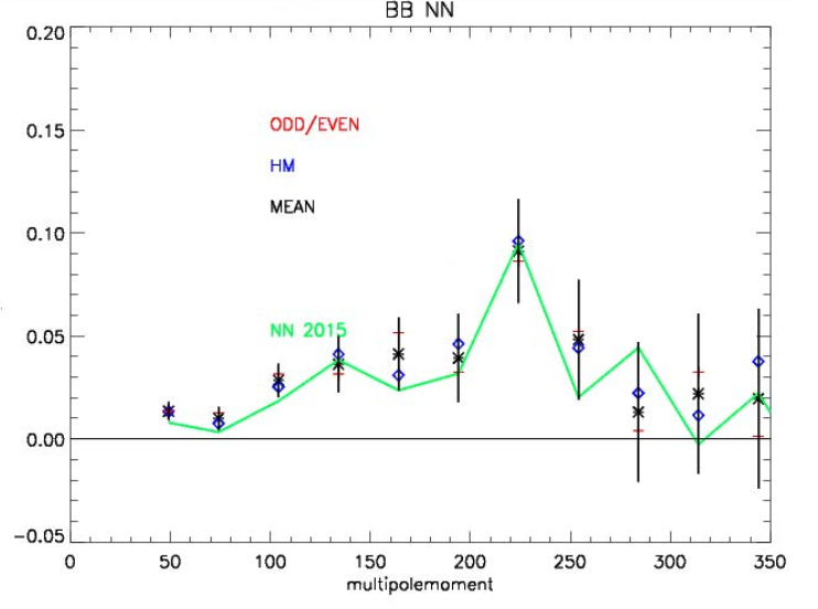
Figure 1: The power of B-mode as a function of multipole moment l. Y-axis: $l(l+1)/2 \pi C_l^{BB} [\mu K^2]$ . Source: Figure 2 in the paper.

To avoid making too many physical assumptions (and possibly biasing the results), scientists have started using neural networks to extract the CMB power spectrum from frequency maps. A neural network is a logic-based, self-training computing method. The neural network’s decision-making process can even evolve for improved decision-making outcomes. Figure 1 shows that using neural networks to extract the B-mode power spectrum from two different maps yields nearly matching results.

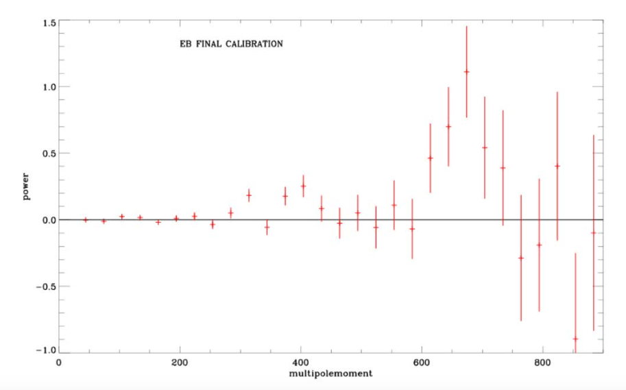
Figure 2: The fully calibrated cross-correlated EB power spectrum. Y-axis: $l(l+1)/2 \pi C_l^{EB} [\mu K^2]$ . Source: Figure 8 in the paper.

Two interesting features appear around l= 675 and l = 375 in the EB cross-correlated power spectrum (Fig. 2). As these features coincide with two peaks in the E-mode power spectrum, it is safe to assume that there is some signal leaking from E to B, estimated around 1 – 2%. This leakage is therefore expected to be an insignificant contribution to the B-mode power spectrum when compared to larger noise sources. Speaking of which…

What about that pesky Galactic noise?

To study the effects of galactic noise in the analysis, the authors analyzed frequency maps at low angular scales, with each map having a different sky coverage. The results are plotted in Figure 3. They conclude that no significant trend can be discovered by varying the amount of sky coverage. In short: galactic noise isn’t a big problem!

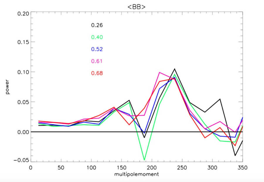
Figure 3: Power spectra with sky coverage factors of 0.26, 0.40, 0.52, 0.61, 0.68. There are no trends as a function of sky coverage. Y-axis: $l(l+1)/2 pi C_l^{BB} [\mu K^2]$ . Source: Figure 10 in the paper.

In conclusion, as our instruments improve and our analysis becomes more robust, our understanding of the universe will only grow, allowing for the fingerprints of gravitational waves to reveal themselves as we peer into the early universe.

About the Author

About Astrobites

This post was written collectively by multiple members of the Astrobites team. Meet the authors of Astrobites.