Welcome to the virtual summer American Astronomical Society (AAS) meeting! Astrobites is attending the conference as usual, and we will report highlights from each day here. If you’d like to see more timely updates during the day, we encourage you to search the #aas238 hashtag on twitter. We’ll be posting once a day during the meeting, so be sure to visit the site often to catch all the news!
LAD Plenary Lecture: Origins of Astrochemical Complexity (by Luna Zagorac)
Astrochemical complexity and its origins is a topic that is just too — well, complex! — to cover in a single plenary. For this reason, Karin Öberg (Harvard University) began with a small amendment to the talk title: she focused on “(Icy) Origins of Astrochemical Complexity (During Planet Formation).” Specifically, she tracked the origins of volatile organic compounds through the process of planet and star formation. In chemistry speak, “volatile” means that these molecules prefer to be in the gas stage, while “organic” means that they necessarily have a carbon (C) atom, often linked to oxygen (O) and nitrogen (N). Understanding where these molecules come from is crucial, because they are the building blocks of life on Earth! But before we can have life, we have to have a planet. The story of planet formation, roughly, is as follows: first, there is a cloud of dust; as this cloud collapses it forms a protostar in the center, and subsequently a protoplanetary disk around it. This system evolves until it begins to look something like our solar system: a central star with (some terrestrial) planets orbiting it, one of which might contain a life-form. But where along this celestial journey did we pick up enough organic volatile molecules to make up said life-form?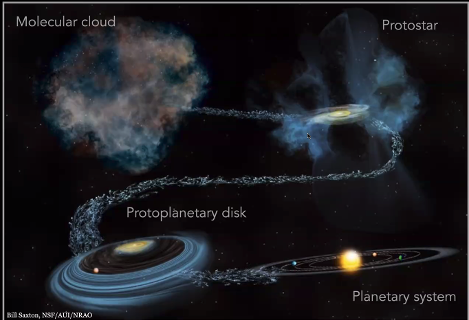
Image illustrating the stages of planetary system formation. [Bill Saxton, NSF/AUI/NRAO]
Press Conference: Molecules in Strange Places (by Tarini Konchady)
The first presentation at this briefing was given by Kate Gold (Bryn Mawr College) and Deborah Schmidt (Franklin & Marshall College). They discussed the preliminary results of a search for molecules around planetary nebulae (PNe). PNe play a key role in determining the chemical content of the interstellar medium, so it’s important to ascertain what molecules can survive the violent irradiation that occurs in the PNe stage. Models suggest that scarcely any molecules make it out intact, but observations point to the opposite being true! Using the 12 Meter Telescope and the Submillimeter Telescope in Arizona, the team searched for signatures of the molecules HCN and HCO+ in 13 PNe of varying ages. Not only did they find significant fractions of these molecules around most of the observed PNe, they also found that the presence of those molecules did not change significantly with PNe age.
A bipolar planetary nebula in the constellation Scutum. [ESA/Hubble & NASA, L. Stanghellini]
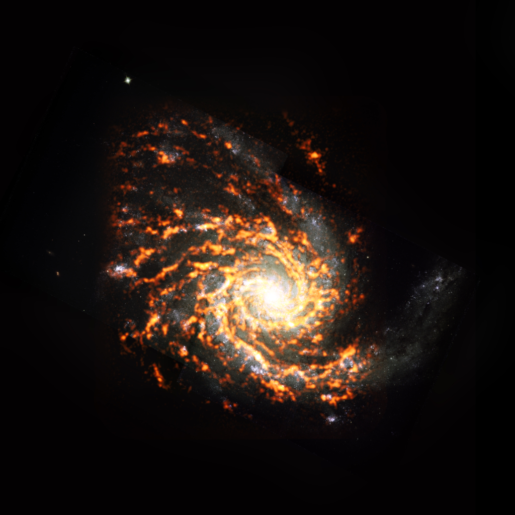
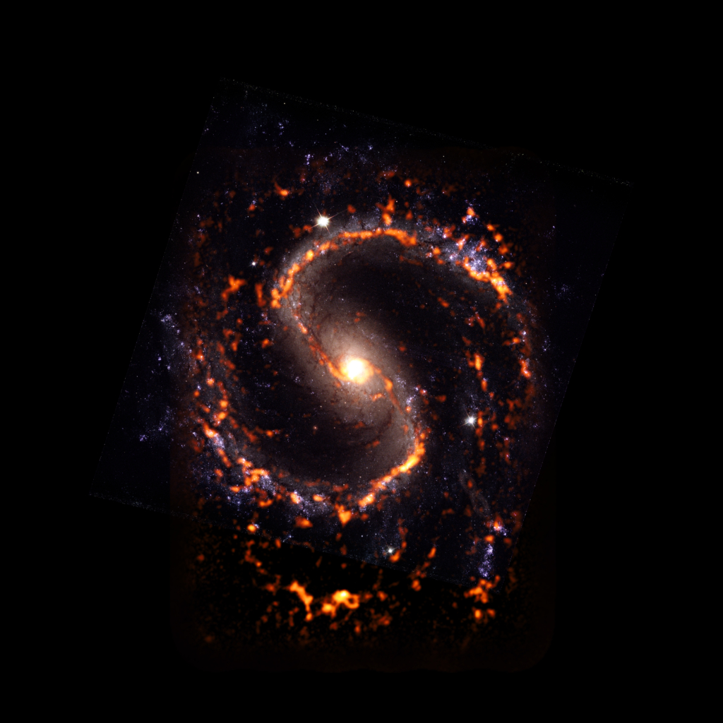
An example of a galaxy surveyed in the PHANGS-ALMA survey. The bright orange regions indicate molecular clouds. [ALMA (ESO/NAOJ/NRAO)/PHANGS, S. Dagnello (NRAO)]
STScl Town Hall (by Sabina Sagynbayeva)
Dr. Nancy Levenson, the deputy director of STScI, reported on the status of the existing and upcoming missions and described new opportunities designed to advance astrophysics through the 2020s. She started off reporting the most recent status of the institute: Most Institute staff are working from home now. More people will return on-site in the coming months, but STScI will not host visitors or conferences in person through the calendar year due to focus on current missions. What missions? Here’s a status update on a few:- JWST is going to launch later this year!
- Hubble’s doing great. Cycle 28 is underway, and the review for Cycle 29 will happen this month. STScI encourages you to share your results if you used Hubble or another telescope supported by STScI, and STScI can help disseminate newsworthy findings. Hubble’s program ULLYSES, a large Director’s Discretionary program for the community to obtain a spectroscopic reference sample of young low- and high-mass stars, put out its second data release in March 2021.
- The Nancy Grace Roman Telescope will provide a Hubble quality with 100 times the field of view. Roman is working toward launch in the mid-2020s. Also, the primary mirror is complete and all WFI science detectors are available. Levenson also reports that ALL data from Roman will be available with zero exclusive access period. Also, Mikulski Archive for Space Telescopes (MAST) can provide data from Hubble, Webb, Roman, Pan-STARRS, and others.
- Space Telescope Users Committee (STUC)
- JWST Users Committee (JSTUC)
- MAST Users Group (MUG)
- Roman Space Telescope Advisory Committee (RSTAC)
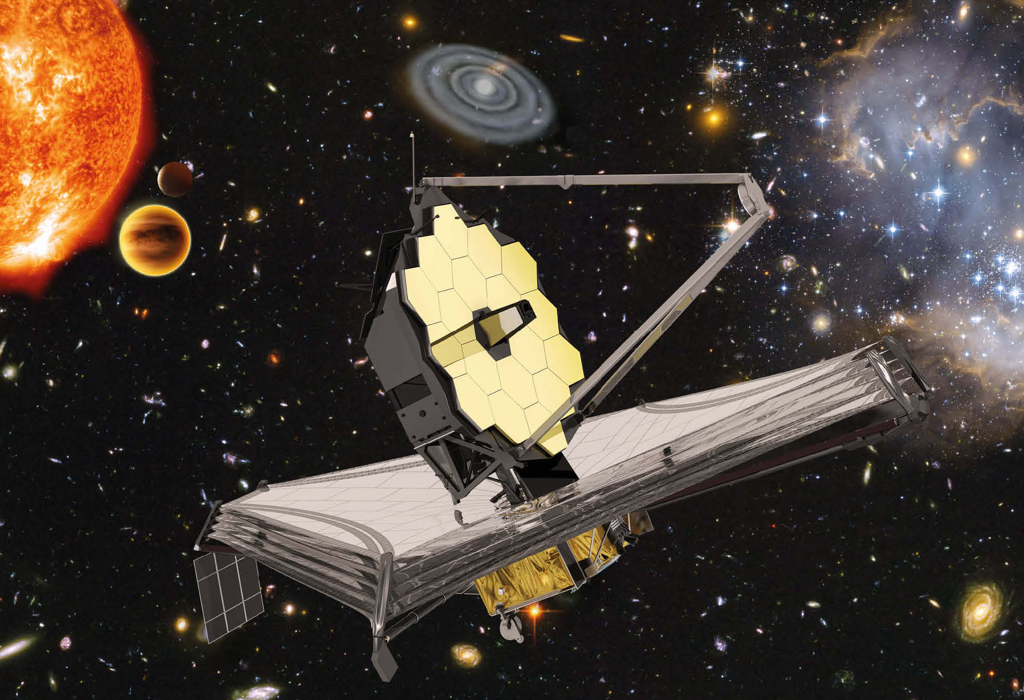
This artist’s impression of JWST highlights the broad variety of science that has been approved for Cycle 1. [ESA, NASA, S. Beckwith (STScI) and the HUDF Team, Northrop Grumman Aerospace Systems / STScI / ATG medialab]
- Protoplanetary disks observations will study the chemistry of water and organics in the terrestrial planet forming regions (<5 AU) and use coronagraphic imaging to search for protoplanets in at least 12 disks
- Transiting exoplanet observations include the study of sub-Neptunes and super-Earths with time-series spectroscopy and planets transiting active M dwarf stars.
- Nearby Galaxy Observations will contribute to understanding of the stellar populations and ISM within nearby galaxies
- AGN outflows and feedback observations will leverage 5–28 µm spectroscopy to determine the heating mechanisms for and estimate the energetics of outflows; characterize the molecular gas, dust, AGN, star formation and metallicity within the central regions; and map the AGN’s influence on the distribution of metals and star formation in different environments
- Galaxy imaging surveys will image the sky using NIRCam (and MIRI), providing the gold-standard imaging data set for galaxy assembly studies, studying the sources responsible for the reionization of hydrogen, and probing the era of the first galaxies, pushing beyond z = 10
- Galaxy spectroscopic surveys will observe thousands of galaxies using NIRCam and NIRISS WFSS to provide line diagnostics reaching redshifts up to z = 7 and beyond, enabling characterization of the physical properties of galaxies all the way to cosmic dawn
Meeting-in-a-Meeting: Transient Discovery with Machine Learning (by Sabina Sagynbayeva)
Gautham Narayan (University of Illinois at Urbana-Champaign) opened the session with “Deep Learning for Multimessenger Astrophysics.” How can we classify sources in the huge volume of photometric data expected in the future? Narayan presents on the Photometric LSST Astronomical Time-series Classification Challenge (PLAsTiCC), a means of using deep learning to classify the time-domain sky. The primary goal? To set up a massive time-domain simulation infrastructure and jumpstart machine learning photometric classification efforts. Andrew Vanderburg (University of Wisconsin-Madison) next talked about “Exoplanet Detection using Machine Learning”. The problem in exoplanet detection is that planets are not the only things that cause stars to dim periodically! We have a lot of data from Kepler and TESS, but we need to identify the dimmings that are specifically caused by planets. Machine learning does two things better than humans: it can perform similar tasks much faster, and it can perform pattern recognition, identifying predictive relationships between different observations that are too complex for traditional methods to solve. Vanderburg presented on how these advantages have been leveraged for exoplanet detection with great success, resulting in multiple potential new planets and the first mass measurement of a known planet around an active star. Michelle Lochner (University of the Western Cape/ South African Radio Astronomy Observatory) next discussed “Transient Classification and Anomaly Detection in the LSST Era.” The Vera Rubin Observatory will produce an incredible dataset, but it is also going to be an incredible challenge. There are rare events that we know exist, e.g. kilonovae, which Lochner calls “known unknowns.” But unknown unknowns are exciting, too! How do we discover new phenomena among 10 million possibilities? An interesting anomaly to one scientist isn’t interesting to another scientist — so here comes active learning. Lochner built Astronomaly, a package for active anomaly detection for astronomical data. By running machine learning algorithms, this pipeline picks up things that are strange and gives an image a score of how “interesting” it is. Lochner concluded by mentioning their mentoring program for women and gender minorities in physics (and they need more mentors!). Ashish Mahabal (Caltech) talked about “Machine Learning Aided Classification of Transients and Variables in ZTF.” The Zwicky Transient Facility (ZTF) has a catalog of billions of astronomical objects and specialized filters depending on science use cases. It registers hundreds of thousands of events every night. Mahabal provided an overview of parts of the machine learning workflow in place to discover and classify transients by combining ZTF photometry and spectra from the SED Machine (SEDM). Guillermo Cabrera-Vives (Department of Computer Science, University of Concepción) wrapped up with “Machine Learning within the ALeRCE System: Past, Present and Future”. ALeRCE is an astronomical alert broker — a system that ingests, processes, and redistributes alerts that come from programs like ZTF — or, in the future, LSST. ALeRCE receives an alert stream about possible transient detections, and then applies machine learning to classify the transient, crossmatch it with archival catalogs, and more.NSF Town Hall (by Macy Huston)
The NSF Town Hall began with updates on Division of Astronomical Sciences (AST) staffing from interim director Chris Smith, followed by updates on observatories and instruments. In recent NOIRLab news, the Dark Energy Survey’s first three years of observations have produced 30 new papers. Meanwhile, the Dark Energy Spectroscopic Instrument (DESI) has completed its trial and begun the five year survey. Exciting news at the Green Bank Observatory is the development of radar capabilities by the NRAO on the Green Bank Telescope. Finally, the Covid-19 pandemic has caused delays and additional expenses in telescope construction. The Daniel K. Inouye Solar Telescope is now estimated to begin operations at the end of 2021. Its Cycle 1 call for proposals will be May 1, 2022, and the start of steady-state observations is anticipated for November 2022. The Vera C. Rubin Observatory is now estimated to begin operation in the first half of 2024.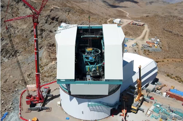
The Vera C. Rubin Observatory, pictured under construction in March 2021. [Rubin Observatory/NSF/AURA]
Annie Jump Cannon Prize Lecture: Turbulent Beginnings: A Predictive Theory of Star Formation in the Interstellar Medium (by Ellis Avallone)
The first afternoon plenary of AAS 238 Day 2 is by Blakesley Burkhart (Rutgers University), winner of the 2019 Annie Jump Cannon Prize! Dr. Burkhart is an expert in turbulence, a complex phenomenon that affects space at a vast range of scales. Her talk begins by first highlighting Annie Jump Cannon herself, whose work in the early 20th century set the stage for the now well-established subfield of stellar evolution. Star formation, however, is an astrophysical process that remains largely unsolved. According to Dr. Burkhart, “We really don’t have a good predictive model [for star formation].” Uncertainties in star formation processes, incidentally, reverberate through all aspects of astrophysics, from galaxy dynamics to planet formation.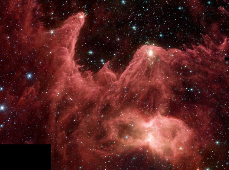
How does the interstellar medium collapse to form stars? [NASA/JPL-Caltech/Harvard-Smithsonian]
Meeting-in-a-Meeting: Measuring the Properties of Stars with Machine Learning (by Mia de los Reyes)
In this session of the “Machine Learning in Astronomy” splinter meeting, we learned about some of the ways data-driven techniques can be used to study stars! Stella Offner (The University of Texas at Austin) started us off by speaking about “Harnessing Machine Learning to Identify Stellar Feedback.” Stars are messy! They inject energy and momentum into their environments, and this feedback can produce all kinds of features in the interstellar medium. Such features, like bubbles and outflows, are often identified visually — but this is time-consuming, subjective, and hard! Offner described an algorithm that instead uses convolutional neural networks to identify these features. After being trained on simulated maps of molecular emission, this algorithm does a great job of finding structures produced by feedback — it’s even been able to show that the feedback in these features scales almost one-to-one with the number of individual young stars in a molecular cloud! Next, Anna-Christina Eilers (MIT) discussed “Mapping the Milky Way with data-driven models.” We live in an era of abundant information about the positions, motions, and spectra of stars in the Milky Way, which can be used to answer open questions about our galaxy’s formation and evolution. But these data have uncertainties! Eilers is using machine learning techniques to derive precise distances and to calibrate stellar abundances. For example, by assuming that red giant branch stars have “standardizable” luminosities, Eilers can use photometric and spectroscopic data to predict their distances with high precision. Similarly, stellar abundances can be predicted using a function of stellar properties. These can be used to make precise maps of stellar velocities and abundances in the Milky Way. Melissa Ness (Columbia University) went more in-depth on stellar abundances with a talk on “Measuring the properties of stars with data-driven computational approaches.” Surveys like APOGEE and LAMOST are providing us with millions of stellar spectra. What information is contained in these spectra, and how can we use them for science? Ness describes how pipelines like The Cannon are able to reproduce stellar spectra with a simple model that includes only a few stellar properties, like effective temperature, surface gravity, and iron abundance. Interestingly, although spectra contain information about many elements, just a few elements (like iron and magnesium) are needed to predict the abundances of other elements. Finally, data-driven techniques can be used to identify stars with outlier spectra, which can help probe the physics of stellar evolution. Lily Zhao (Yale University) also discussed stellar spectra, but focused more on measuring radial velocities rather than abundances. In the talk “Machine Learning for Extreme Precision Radial Velocity,” Zhao explained that in order to discover an Earth-like planet using radial velocities, we’d need a spectrograph with around 10 cm/s precision. Next-generation spectrographs can reach sub-m/s precision, but spectroscopic effects from stellar activity become a significant source of error. This is where machine learning comes in! Data-driven techniques can effectively reduce the impact of stellar activity on radial velocity measurements.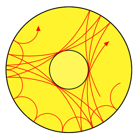
Asteroseismology uses different oscillation modes of a star to probe its internal structure and properties. [Tosaka]
LAD Laboratory Astrophysics Prize: Tales from a Life in Laboratory and Observational Molecular Astrophysics (by Luna Zagorac)
The winner of the AAS LAD Laboratory Astrophysics Prize, Geoffrey Blake (Caltech), looked back on a long career of astrochemical achievements in his talk. The Blake group at Caltech focuses on spectroscopy, spanning the range from microwave to infrared and near-optical frequencies. This is equivalent to a range in temperatures from a few to a few thousand Kelvin, allowing them to probe a wide variety of molecular motions in the sky. Blake emphasized the exquisite quality of ALMA data for astrochemistry, noting that his group worked on laboratory instrumentation to bring it in step with the quality and quantity of observational data. On the other hand, the opposite is true when studying chiral molecules with three dipole moments: they are very-well understood in the lab, but they would require circularly polarized light sources in the sky imaged with an instrument at least the size of the Square Kilometre Array to study observationally. Finally, he highlighted how Spitzer data allows us to study ices and gases (including water!) in planetary formation contexts. He closed out his talk with acknowledgements of both his mentors and past and current students and postdocs, noting particularly how lucky he was to become a Duke Microwaver during his time at Duke University, which ultimately led him to discovering his own astrochemical path. Live-tweeting of the session by Luna ZagoracLAD Dissertation Prize: Oxygen Insertion Chemistry: A Low-temperature Channel to Organic Molecule Production (by Luna Zagorac)
The graduate thesis written by Jenny Bergner (University of Chicago) was instrumental in the discovery of a new pathway for complex molecules to form in the icy interstellar medium (ISM): it’s no wonder that she won the LAD Dissertation Prize! Recreating the conditions of the ISM in the lab (a temperature of about 10 K and pressure many orders of magnitude below atmospheric), Bergner was able to use infrared spectroscopy to monitor what happened to icy molecules under these conditions. Turns out, an oxygen singlet state (a form of oxygen atom denoted as O(1D)) is able to insert itself directly into the bond between a carbon and hydrogen atom, forming new organic compounds in a process called O-insertion. The kicker? It’s able to do this without any energy input — meaning, it could even happen in the harsh conditions of the ISM! This process leads to fragmentation, meaning that new but less complex molecules are produced. However, this is true of so-called saturated hydrocarbons, with a single bond between the C and H atom. In unsaturated hydrocarbons, which might have double or triple bonds between two carbon atoms, an analogous process called O-addition can take place, again with no energy input. Thus, O-insertion and O-addition are able to account for much of the astrochemical complexity seen in ISM ice. Furthermore, no other mechanism can explain the production of ethylene oxide (which has been detected in the ISM). Finally, Berger talked briefly about the role of comets in transferring ISM ices into protoplanetary systems. Small grains could not survive this journey, but larger ones were found to experience virtually no loss on this journey. Interview of Jenny Bergner by Luna Zagorac Live-tweeting of the session by Luna ZagoracSPD Harvey Prize Lecture: A Journey from Quiet Sun Magnetic Fields to Flares (by Sabina Sagynbayeva)
The SPD/AAS early career Karen Harvey Prize is awarded in recognition of a significant contribution to the study of the Sun early in a person’s professional career. This year’s winner, Lucia Kleint (University of Geneva), got into research on solar flares accidentally, but she continues to investigate their inner workings today while also trying to understand how to improve solar observations!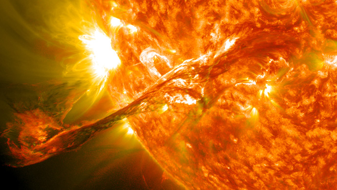
What types of stars are most likely to host stellar flares like this one, emitted by our own star and imaged by the Solar Dynamics Observatory? [NASA/GSFC/SDO]
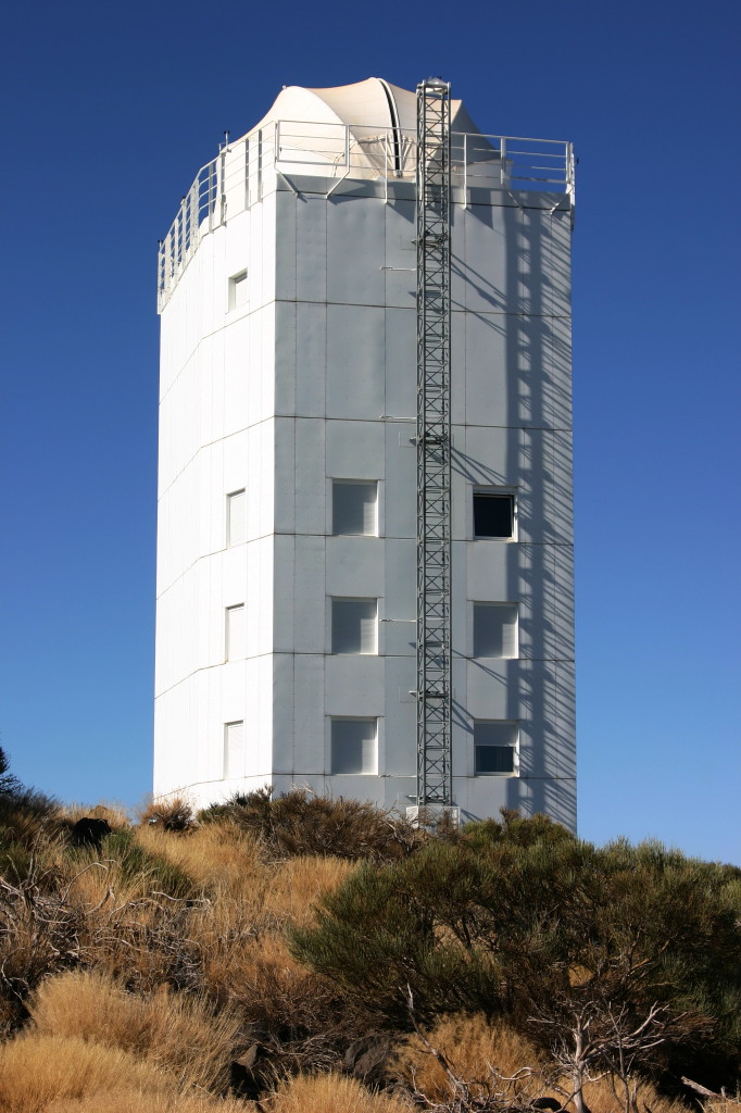
Solar Telescope GREGOR at the Teide Observatory, Tenerife, Canary Islands. [H. Raab
- So far, we have no regular high-resolution chromospheric magnetic field measurements. Do we need DKIST, or a spacecraft?
- Advances in flare modeling and analysis (Radyn, RH, STIC, machine learning)
- Automatic analysis of millions of spectra/images, which may enable flare prediction
Seminar for Science Writers: Get Ready for Webb! (by Tarini Konchady)
Christine Pulliam and Hannah Braun (Space Telescope Science Institute) introduced this seminar, which is intended to give an overview of the James Webb Space Telescope (JWST) and the science it will do. First, Eric Smith (NASA Headquarters) provided a description of the final months before JWST’s expected launch and the commissioning that will follow. The telescope continues to be tested to ensure it will work after launch, and the Cycle 1 observing programs have been announced (see the summary of the STScI town hall). Following launch, JWST will see a roughly 180-day commissioning, during which it will ready itself to observe. This process includes the deployment of the telescope mirrors and the calibration of the scientific instruments on board. Cooling is also a critical part of this process, since JWST will be observing in the infrared.
The path of light along JWST’s mirrors as it is directed towards the scientific instruments. [STScI]
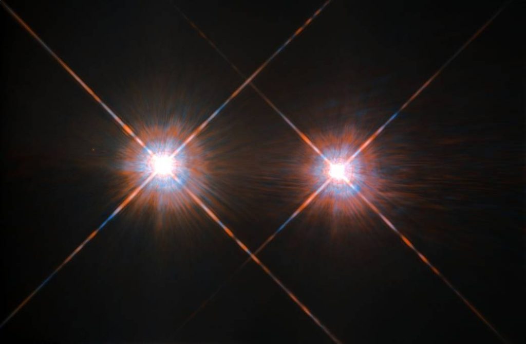
Alpha Centauri A (left) and B (right) as seen by the Hubble Space Telescope. JWST will search for exoplanets around Alpha Centauri A. [ESA/NASA]
Plenary Lecture: Our Galaxy in Context: Satellite Galaxies around the Milky Way and Its Siblings (by Mia de los Reyes)
Marla Geha (Yale University) wrapped up Day 2 of #AAS238 by discussing the “nieces, nephews, and niblings” of the Milky Way: the low-mass satellite galaxies around Milky Way-like galaxies! Why focus on these small galaxies? The ~60 known satellite galaxies around the Milky Way are useful laboratories for testing theories about cosmology and galaxy formation.
The title screen from Marla Geha’s plenary talk, showing many of the satellite galaxies identified by the SAGA survey.