Authors: Michael Boylan-Kolchin
First Author’s Institution: Dept. of Astronomy, The University of Texas at Austin, Austin, TX
Status: Submitted to MNRAS, open access
In the past we’ve covered a few potential sources for the reionization of the universe, such as AGN or supernovae. It is believed that the primary contributor of UV radiation during reionization was from the earliest formed galaxies (think redshift z ~ 12). Therefore it can be really informative to understand how these galaxies are producing their UV flux. So for today’s astrobite we look into what ancient globular clusters were doing during the epoch of reionization (z ~ 6-10).
What are globular clusters?
To understand how globular clusters (GCs) can contribute to reionization, we need to understand some background about them. Globular clusters are gravitationally tightly-bound, spherical, ex-star-forming regions within galaxies. These very dense stellar clusters orbit fairly close to the galactic center, and usually contain some of the earliest formed stars in that galaxy. This means that in the early stages of galaxy formation globular clusters should have contributed a sizable amount to the high redshift UV luminosity output. You can read more about how GCs form in this astrobite.
Learning from the GC luminosity function
Now we have a basic idea of what GCs are, but how can we use this knowledge to predict how important they were during reionization? By using the GC UV luminosity function of course! The GC UV luminosity function (or GC UVLF) gives the number of GCs per volume per luminosity and this function evolves with redshift. They use the UV luminosity function in particular because the majority of photons that re-ionize neutral hydrogen will have UV wavelengths.
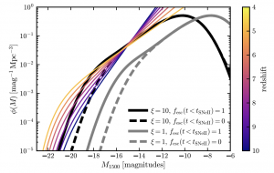
Figure 1: Observed global UVLFs from the Hubble Space Telescope (in color) as compared to the observed GC UVLFs. This plot demonstrates how much GCs contribute to the global UVLF. Depending on parameters such as the escape fraction, [latex]f_{esc}[/latex] or the ratio of stellar mass from birth to now, [latex]\xi[/latex], these can affect the UVLF by reducing the number of bright GCs (more negative) or create a more steep bright end slope (difference between solid and dotted).
The author of today’s astrobite uses the current (z=0) number density of GCs and the stellar mass function to extrapolate backwards to the reionization era. In doing this, they assume a log-normal fit to describe the initial GC stellar mass function, which ultimately gives a log-normal distribution for the GC UVLF. They then compare the GC UVLF to the global UVLF at high redshifts. This becomes a bit complicated as the derived luminosity function is an intrinsic GC UVLF, meaning it’s unobscured by any material such as dust or gas. In an attempt to make the best comparison they transform the intrinsic GC UVLF into an observed GC UVLF. This is done by using the escape fraction, \(f_{esc}\), which describes the amount of UV radiation that makes it beyond the GC. To apply a time scale to \(f_{esc}\), the author uses the time that it takes for type-II supernovae to remove the gas surrounding GCs leaving UV radiation free to travel.
The observed GC UVLFs in comparison to the global UVLFs (see Fig. 1) do in fact prove to be a considerable component of the global UVLF. This is even easier to see in Fig. 2, which shows the ratios of the two quantities for different redshifts. They additionally look at two distinct models (\(\xi = 1, 10\)) which is the ratio of stellar mass at birth compared to now. These \(\xi\)’s give us two points of interest where the stellar mass remains the same, \(\xi = 1\), and where the stellar mass at birth is an order of magnitude larger, \(\xi = 10\).
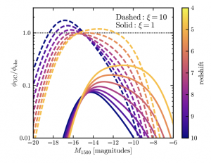
Figure 2: The ratio of GC to global UVLFs. The GCs where the initial stellar mass to current stellar mass, [latex]\xi[/latex] = 1, show a contribution of at least 10% at all redshifts!
One caveat the author points out, is that in the UVLFs shown in Fig. 1, we cannot expect the \(\xi\) = 10 distributions to be realistic in this model. This is because the increase in bright GCs to the point of being 100% of the global UVLF would have already been detected, thus we should expect \(\xi < 10\). Therefore this means we now have potentially more constraints on GCs during reionization or we may need an alternative way to model the GC UVLF over redshift. Once the James Webb Space Telescope (JWST) is up and running we’ll be able to push the envelope on potentially detecting GCs earlier in their lives. This would give us an improved understanding of ones closer to the epoch of reionization.
Author
Trackbacks/Pingbacks