Title: Measuring the star formation rate with gravitational waves from binary black holes
Authors: Salvatore Vitale & Will M. Farr
First Author’s Institution: LIGO, Massachusetts Institute of Technology, Massachusetts, USA; Kavli Institute for Astrophysics and Space Research, Massachusetts Institute of Technology, Massachusetts, USA
Status: Submitted to arXiv, open access
Our first detection of gravitational waves with LIGO changed everything for astronomy. For the first time, we are able to not just look out into the Universe, but “listen” to it as well. So far, we’ve heard the collisions of the remnants of massive stars: black holes and neutron stars. The resulting data has had massive implications in fields from general relativity to nucleosynthesis. Today’s paper proposes a new use for detections of binary black hole (BBH) mergers. Vitale & Farr (2018) make the argument that if we know how often black holes are colliding, we should be able to determine how often stars form to produce these black holes.
Star formation and black hole death
The star formation rate (SFR) in a galaxy is a crucial variable for interpreting the brightness of a galaxy. Different galaxies that formed at the same time will have similar SFRs, but as the universe ages the star formation rate changes. In the earliest stages of the Universe, stars have not had time to form yet. After too long, however, star formation is “quenched” by various processes that eject the necessary gas from the galaxy. Figure 1 shows that the star formation rate peaked at redshift z=2 (about 10 billion years ago) but it also demonstrates that we have significantly less data at higher redshifts (further back in time). Part of the difficulty in measuring distant SFRs is the large amount of dust in the way. Since gravitational waves are unaffected by dust, the authors of today’s paper argue that gravitational waves have a significant advantage in probing the early universe.
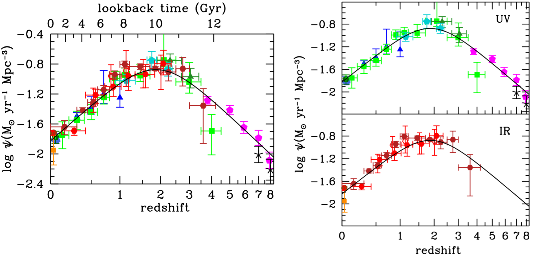
Figure 1: Star formation rate versus redshift measured with FUV light (top right panel), IR (bottom right panel), and the two combined (left panel). The points were determined by past surveys. Different colors correspond to different surveys. Figure 9 in Madau & Dickinson (2014).
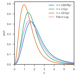
Figure 2: Probability distributions of BBH merger events versus redshift. The “Flat in Log” curve considers a case where it is equally likely that a BBH merger occurs any time between 10 million and 10 billion years post-formation. Figure 1 in the paper.
Of course, just because a star forms does not mean it will be a part of a BBH merger. These events are relatively rare. The authors point to calculations that as few as 10,000 mergers occur in the entire observable universe per year. Also, even for the largest and shortest lived stars this cataclysmic end will follow formation only after a significant amount of time. Characterizing this delay, which accounts for the stellar lifetimes and eventual orbit decay, presents a reasonable challenge. The authors therefore consider a variety of different functions to describe how likely a merger event is at different redshifts with the parameter τ given as the e-fold time for BBH mergers after stellar formation (Figure 2). Using this information, combined with a fit of SFR versus redshift based on Figure 1, the authors model BBH mergers as a Poisson process and simulate 15,000 events.
Results

Figure 3: The merger rate versus redshift. Dashed lines are the “true” simulated rates while the solid lines are the rates determined using the second fitting approach. Shading around the solid lines indicate one sigma (dark color) and two sigma (light color) errors. The “prompt” line corresponds to analysis where τ -> 0. Figure 2 in the paper.
With the simulated data, the authors model the BBH merger rate using two different fitting approaches. With the first, they pretend to know nothing about the underlying SFR and simply create piecewise functions to describe the merger rate versus redshift. For the second fit, they use the same functional forms used to generate the data and they try and extract the original parameters used in the SFR and the time-delay scale, τ. Both fits successfully described how often mergers were simulated (Figure 3), and the second process recovered almost all parameters within a single standard deviation. While it was generally more difficult to match the merger rates at high redshifts, this is partially because there are fewer events (less time has passed for stars to form and die) and because the simulated data only allowed mergers to occur after 100 million years for computational purposes.
A key point in the paper is that the high precision measurements of the SFR parameters required only a month’s worth of data. The authors admit that they used a relatively simple model for the SFR (for example, they did not vary it with mass) but are confident that large data sets would enable more complicated modeling. Such large data sets might be in the foreseeable future. At the beginning of today’s paper, the authors point to the upcoming third generation of gravitational wave detectors including the Einstein Telescope and the Cosmic Explorer. These extremely high precision gravitational wave detectors could observe BBH mergers at far redshifts but they are still in their very early stages of development. Still, with the immense success of LIGO further developments in gravitational wave detectors seem inevitable. Gravitational waves have unlocked an entirely new paradigm of observing the Universe, and as today’s paper demonstrates the astronomy community is well prepared to apply those observations across the entire field.
References
- P. Madau and M. Dickinson, “Cosmic Star-Formation History,” Annual Review of Astron and Astrophys 52, 415–486 (2014), arXiv:1403.0007.
Author
Thanks for that Avery. As a “senior” physicist wannabe, I can’t quite disentangle the SFR concept outlined here, and the total star formation going back to the birth and condensation of the galaxy. At that time the SFR must have been hundreds or thousands of solar mass stars per year in order to account for the typical 100 billion stars alone in the MW. So how is the SFR concept in the paper disentangled from the “total” star formation rate during the formation of the galaxy?
Hi George, thank you for the question! I agree that there is an important distinction between the SFR discussed in this article and a galaxy’s “local” SFR. My apologies for not stressing that distinction more in the article.
I think the key point is that this work is trying to measure the stellar formation rate *density* (notice the units in Figure 1). These values therefore describe the SFR averaged across entire sections of the Universe at a given redshift. Since a large amount of this volume will be empty space, rather than star forming galaxies, the SFRs will be significantly smaller than what we see in galaxy formation. A quick order of magnitude calculation (the volume of the Milky Way is ~1e61 meters) suggests that even at the peak SFR in Figure 1, the Milky Way would produce less than 100 solar masses in a billion years. Obviously this can’t be correct!
While the stellar formation rate density (I’m seeing SFRD used in some cases) effectively erases the information about individual galaxies, it does tell how us SFRs should change with time. It can’t give us the SFR for a given galaxy, but it can tell us when that rate was likely increasing or decreasing throughout the galaxy’s history.
Thanks. Yes, I see. We get How SFR can change over time, but not SFR for a particular galaxy.